Estimating the power to detect a change caused by a vaccine from time series data

Daniel M. Weinberger; Joshua L. Warren

doi:10.12688/gatesopenres.13116.1

Home Browse Estimating the power to detect a change caused by a vaccine from time...

ALL Metrics

Views

Downloads

Get PDF

Get XML

Export

▬

✚

Research Article

Estimating the power to detect a change caused by a vaccine from time series data

[version 1; peer review: 1 approved, 1 approved with reservations]

Daniel M. Weinberger ^1,2, Joshua L. Warren^2,3

PUBLISHED 09 Mar 2020

Author details Author details

¹ Department of Epidemiology of Microbial Diseases, Yale School of Public Health, New Haven, CT, 06520, USA
² Public Health Modeling Unit, Yale School of Public Health, New Haven, CT, 06520, USA
³ Department of Biostatistics, Yale School of Public Health, New Haven, CT, 06520, USA

Daniel M. Weinberger
Roles: Conceptualization, Formal Analysis, Funding Acquisition, Methodology, Software, Visualization, Writing – Original Draft Preparation, Writing – Review & Editing

Joshua L. Warren
Roles: Methodology, Writing – Review & Editing

OPEN PEER REVIEW

REVIEWER STATUS

Abstract

When evaluating the effects of vaccination programs, it is common to estimate changes in rates of disease before and after vaccine introduction. There are a number of related approaches that attempt to adjust for trends unrelated to the vaccine and to detect changes that coincide with introduction. However, characteristics of the data can influence the ability to estimate such a change. These include, but are not limited to, the number of years of available data prior to vaccine introduction, the expected strength of the effect of the intervention, the strength of underlying secular trends, and the amount of unexplained variability in the data. Sources of unexplained variability include model misspecification, epidemics due to unidentified pathogens, and changes in ascertainment or coding practice among others. In this study, we present a simple simulation framework for estimating the power to detect a decline and the precision of these estimates. We use real-world data from a pre-vaccine period to generate simulated time series where the vaccine effect is specified a priori. We present an interactive web-based tool to implement this approach. We also demonstrate the use of this approach using observed data on pneumonia hospitalization from the states in Brazil from a period prior to introduction of pneumococcal vaccines to generate the simulated time series. We relate the power of the hypothesis tests to the number of cases per year and the amount of unexplained variability in the data and demonstrate how fewer years of data influence the results.

Keywords

time series analysis, program evaluation, vaccine evaluation, power calculation

Corresponding author: Daniel M. Weinberger

Competing interests: DMW has received consulting fees from Pfizer, Merck GSK, and Affinivax for work outside of this manuscript. JLW has no conflicts to disclose.

Grant information: This work is supported by the Bill and Melinda Gates Foundation [OPP1176267]; and the National Institute of Allergy and Infectious Disease [R01AI123208; R01137093].
The funders had no role in study design, data collection and analysis, decision to publish, or preparation of the manuscript.

Copyright: © 2020 Weinberger DM and Warren JL. This is an open access article distributed under the terms of the Creative Commons Attribution License, which permits unrestricted use, distribution, and reproduction in any medium, provided the original work is properly cited.

How to cite: Weinberger DM and Warren JL. Estimating the power to detect a change caused by a vaccine from time series data [version 1; peer review: 1 approved, 1 approved with reservations]. Gates Open Res 2020, 4:27 (https://doi.org/10.12688/gatesopenres.13116.1) First published: 09 Mar 2020, 4:27 (https://doi.org/10.12688/gatesopenres.13116.1) Latest published: 19 Oct 2020, 4:27 (https://doi.org/10.12688/gatesopenres.13116.2)

Introduction

After a new vaccine is introduced, it is often necessary to evaluate the effect of the intervention on disease rates. This is typically done by evaluating changes in the average number of cases or the trend in cases before and after vaccine introduction¹. However, this type of analysis is challenging because it can be difficult to distinguish changes in disease rates caused by the vaccine from changes resulting from random variations, epidemics, changes in healthcare utilization, or changes in reporting practices. Additionally, there is often no ‘ground-truth’ against which estimates can be compared to determine whether an estimate is credible. These issues are a threat to the validity of any vaccine evaluation study, even when using large nationwide databases. However, the problems are especially acute when moving from larger to smaller populations, where the signal to noise ratio will be lower.

While it is intuitive that having more noise in the data makes it more difficult to detect a change, it is not clear how much data are needed to effectively quantify a vaccine-associated change if one exists. The power to detect a decline will depend on many factors, including the magnitude of the expected effect (higher power with a greater expected decline), the number of cases per unit time, and the number of years of pre- and post-vaccine data. Because the specific characteristics of datasets can vary, it is difficult to make general statements about power. However, simulation-based methods can be used to evaluate and compare power in different datasets based on the pre-vaccine time series and the magnitude of the expected effects^2,3.

In this study, we present a simple web-based tool that can be used to input any disease time series and obtain an estimate of the power for that series to detect a specified vaccine-associated decline. This is accomplished by extracting characteristics of the time series (e.g., seasonality, trends, unexplained variability) from the pre-vaccine period and simulating a set of time series that have similar characteristics and have a vaccine impact that is specified a priori. We demonstrate the application of this approach on observed pre-vaccine data on pneumonia hospitalizations from the 26 states plus the federal district in Brazil and relate characteristics of the time series to the power.

Methods

Data

We used state-level hospitalization data from Brazil, which have been described in detail previously⁴. These de-identified data are drawn from the Unified Health System (SIH-SUS, Ministry of Health), which captures ~70% of the population in Brazil. The raw data can be obtained directly by contacting the Ministry of Health in Brazil. The formatted time series data are available in the Github repository for this study. Each hospitalization is assigned a unique ICD10 code. For these analyses, we focused on data on <12 month old children and 80+ year old adults for the pre-vaccine period 2003–2009. These two populations provide a useful contrast. The time series for the infants was relatively stable prior to vaccine introduction, while the data for the 80+ year old adults had a notable increasing trend before vaccine introduction. Both sets of time series exhibit strong seasonality with a peak in the winter.

Simulating data based on observed time series from Brazil

The goal for this exercise was to simulate a set of time series with characteristics that resembled the observed hospitalization data from the pre-vaccine period but that had specified vaccine effects added in. We then sought to estimate the vaccine effect using the same model that was used to generate the data and evaluate the power to detect the effect. This provides a best-case scenario where the underlying model is correctly specified.

The first step in this process was to extract characteristics of the time series from the pre-vaccine period (trend, seasonality, and amount of unexplained variation). For each state, we fit a regression model to the data from the pre-vaccine period (2003–2009). The outcome variable was the number of pneumonia hospitalizations (coded as J12-18) per month, and the covariates were an index variable for time (to capture any linear trends in the data) and 12-month and 6-month harmonic variables (to capture seasonality). We used a Poisson regression model with a Gaussian observation-level random intercept to account for overdispersion in the data such that

Y_{t} \sim Poisson (e^{μ_{t} + ϕ_{t}}),

μ_{t} = β_{0} + β_{1} * {time}_{t} + β_{2} * sin (θ_{t} / 12) + β_{3} * cos (θ_{t} / 12) + β_{4} * sin (θ_{t} / 6) + β_{5} * sin (θ_{t} / 6), and

θ_{t} = 2 * π * {time}_{t}

The models were fit using the glmer function in the lme4 package in R, version 3.6.1.

The next step is to use the fitted model to simulate time series of counts of hospitalization with similar characteristics that covered both the pre- and post-vaccine period, with a specified vaccine-associated decline added to the simulated data. Using the estimated regression coefficients $({\hat{β}}_{k})$ and their estimated variance/covariance matrix, we generated 500 independent random draws of the parameters from a multivariate normal distribution for each state and age group combination. These were combined with the design matrix to obtain simulated ${\hat{μ}}_{t} .$ Random draws of ${\hat{ϕ}}_{t}$ were independently generated from a normal distribution with a mean of 0 and a standard deviation equal to the standard deviation estimated for ϕ_t from the fitted model. To incorporate a known vaccine effect, we assumed that the time series declined by a specified amount over a 24-month period. We generated time series where the maximum vaccine effect after 24 months ranged from a 10% – 50% reduction (rate ratio of 0.5–0.9). To capture these declines, we generated a vector, v_t, with entries equal to 0 prior to vaccine introduction and decreasing linearly to the log(Rate-Ratio-Final) over 24 months. Simulated counts, Y_t,sim, were generated by taking a random draw from the Poisson distribution with mean $e^{{\hat{μ}}_{t} + {\hat{ϕ}}_{t} + v_{t}} .$ The simulated counts reflect uncertainty in the regression parameters, unexplained variability in the data, as well as uncertainty from the observation process.

Estimation of vaccine effects

We next used a regression model similar to the one used to generate the data to estimate the vaccine effect. The outcome was the (simulated) number of counts per month. As above, we adjusted for seasonality using 6- and 12-month harmonic terms, and secular trends were captured using an index for time. The vaccine effect was quantified using a linear spline term that began at the time of vaccine introduction and continued for 24 months before stabilizing. An observation-level random intercept was included to capture overdispersion of the count data. Using the fitted model, we calculated the estimated rate ratio 24 months after vaccine introduction as 24*(coefficient for the vaccine effect term). To evaluate how many years of pre-vaccine data are needed to estimate the effects, we sequentially removed the first 1, 2, or 3 years of data and evaluated the effect on power.

Data and availability

All of the time series data and code used in these analyses are available from a Github repository https://github.com/weinbergerlab/PoissonITS_power. The interactive tool, along with a sample dataset, can be accessed at https://weinbergerlab.shinyapps.io/ITS_Poisson_Power.

Results

Interactive tool to estimate power

Because the power to detect a change in a time series is influenced by the expected effect size, the amount of unexplained variation in the data, and the number of years of data available, it can be difficult to make general statements about power. However, observed time series from the pre-vaccine period can be used to simulate time series to perform a best-case power calculation. This can provide an indication of whether it is worth performing an analysis or whether collecting additional data (e.g., additional pre-vaccine time points) could be helpful. We provide a simple ‘point-and-click’ interface where the user provides a time series in a csv or Excel format, indicates which columns contain the date variable, the outcome, and any potential controls, and the date at which the intervention is introduced (Figure 1).

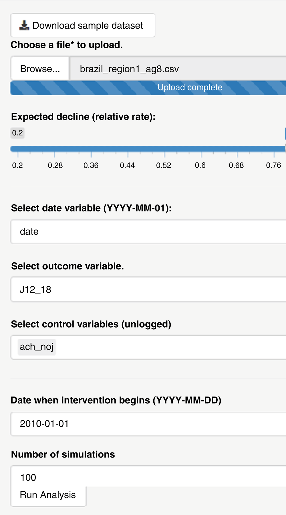
Figure 1. User interface for power calculation.

The user uploads a time series, specifies the expected decline in terms of a rate ratio, specifies the key variables (date, outcome of interest, and controls), the date of the intervention, and the number of simulations to generate. A sample dataset can be downloaded by clicking the button at the top of the screen.

Characteristics of the state-level data from Brazil

As a demonstration of this approach, we apply this simulation framework to data from Brazil, disaggregated to different subnational levels (state, region). The size of the population varies drastically by state, from 450,000 to 41 million individuals (in 2010). On average there were 30-1900 hospitalizations due to pneumonia per month per state among children <12 m and 12-1100 hospitalizations per month per state among adults 80+ years of age during the pre-vaccine period. The time series for the <12m old children were highly seasonal but without a strong long-term trend, while the time series for the 80+ year olds increased markedly starting in the pre-vaccine period. We simulated time series for each of the states that had similar characteristics to the observed time series in the pre-vaccine period but with vaccine effects of different magnitudes (Figure 2).

Figure 2.

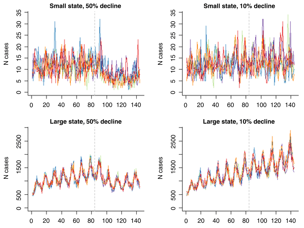
Sample simulated monthly time series of hospitalizations due to all-cause pneumonia for adults 80± years of age from a small state (A,B) and a large state (C,D) in Brazil with a 50% decline post-vaccination (A,C) or 10% (B,D).

Effect of number of cases and random noise on ability to accurately to detect a decline

We first evaluate the relationship between the amount of unexplained variability in the data and the ability to accurately estimate the effect of the vaccine. There is a clear relationship between the amount of unexplained variability in the data and the power to detect a vaccine-associated change (Figure 3A). This trend was consistent across all of the states between both children and adults.

Figure 3.

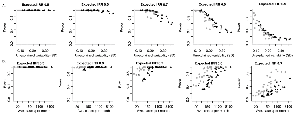
Relationship between power to detect a decline associated with vaccine introduction and (A) the amount of unexplained variation in the time series or (B) the average number of cases per month for different specified magnitudes of vaccine effects. The labels at the top of the panel indicate the magnitude of the expected vaccine effect, with an incidence rate ratio (IRR) of 0.5 representing a 50% decline associated with the vaccine and a IRR of 0.9 equal to a 10% decline. Each dot represents the power for one state in Brazil. The black triangles represent estimates for adults 80+ years of age, and the gray circles represent estimates for children <12 months of age.

Plotting the estimated power against the average number of hospitalizations in the state/region, there is also a relationship, but the trend differed between children and adults (Figure 3B). This is because the amount of unexplained variability was higher in the <12m old children than in the 80+ year old adults (Extended data: Figure S1)

Effect of number of years of data on ability to accurately to detect a decline

With fewer years of baseline data, the power to detect a change in disease rates associated with the vaccine also declines. For datasets with little unexplained variability, even with just 12 months of pre-vaccine data, there could be high power to detect a vaccine-associated decline of 20%. However, when there is more unexplained variability in the time series, power declines with shorter pre-vaccine periods (Figure 4). These declines in power are particularly dramatic for time series with intermediate levels of unexplained variability (Figure 4).

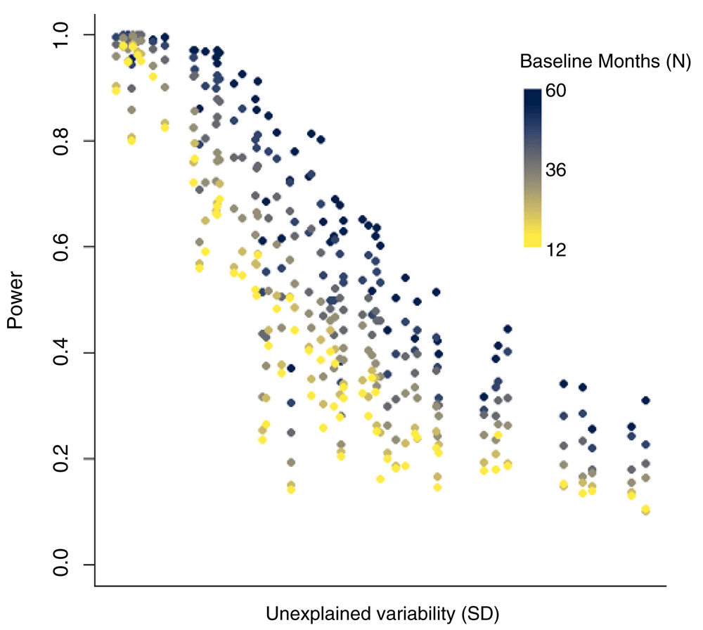
Figure 4. Effect of shortened baseline periods on the relationship between the power to detect a decline associated with vaccine introduction and the amount of unexplained variation in the time series.

Each dot represents the power for one state/age group in Brazil. Dots with lighter colors had fewer years of data.

Demonstration of the interface

As a demonstration of the point-and-click interface, we use hospitalization data from Chile among children <24 months (raw data available from http://www.deis.cl/)⁵. This sample time series can be downloaded directly from the interface. The outcome variable is the number of hospitalizations per month due to all-cause pneumonia (J12_18) for 2003–2014. The number of non-respiratory hospitalizations per month (ach_noj) is included as a control. If no control is present, this field can be left blank. The date of vaccine introduction is set to January 1, 2011. The program generates a specified number of simulated time series (N) based on the pre-intervention data (Figure 5A). With three years of post-vaccine data (vaccine introduction in 2011, evaluating through 2014), the 100 estimates of the rate ratio are centered on the true value (indicated by a red dashed line), with a moderate degree of uncertainty (Figure 5B). This yields 54% power to detect a rate ratio of 0.8 (Figure 5B). Compared with the analyses of the Brazil series, the power is reasonable given the amount of unexplained variability in the data but could be increased (Figure 5C). This can be seen in the simulation by increasing the length of the evaluation period by a year (e.g., in this instance moving the date of vaccine introduction earlier by 12 months to January 2010, which also shortens the baseline period) (Extended data: Figure S2). The power in this instance would increase from 54% to 77% with an improvement in the precision of the estimates. This also highlights that the total number of years of data is not the only key component—it is how that data points are balanced between the pre- and post-intervention periods—too few data on either side will reduce power.

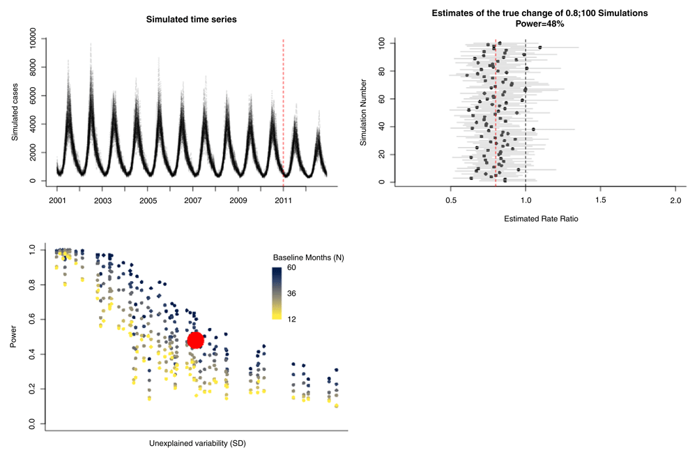
Figure 5. Sample output from the interactive interface using hospitalization data for Chile under 2 years of age (data can be obtained by clicking the download button on the interface).

The upper left panel shows the 100 simulated time series. The upper right panel shows the estimates of the rate ratio for each of the 100 simulations. The true specified rate ratio (0.8) is denoted by a red dashed line. 54% of the estimates had 95% confidence intervals that did not cross 1. The bottom left panel shows the estimate of power for this study (red dot) compared with the estimates from the Brazil states with different length baseline periods.

Discussion

In this study, we describe a simple interface for conducting simulations to evaluate the power to detect a vaccine-associated decline from time series data. This approach provides analysts a simple best-case scenario for determining whether they are likely to detect specified vaccine effects with the data on hand or whether collecting additional pre- or post- vaccine data would be beneficial. This type of tool should be used when planning analyses and prior to conducting a formal evaluation analysis with the data on hand.

By analyzing subnational data from Brazil, we demonstrate how power varies with the number of cases and the degree of unexplained variability in the data. Reducing unexplained variability in the data by using time-varying covariates can help to increase power. Such covariate could include other causes of disease/hospitalization/death or known correlates of changes in disease rates (e.g., percent of the population with access to healthcare).

These analyses evaluate power based on the statistical characteristics of the time series. As with any analysis, failure to correctly control for relevant trends will also introduce important biases and could greatly outweigh the issues related to statistical characteristics of the data. For instance, if there is a non-linear trend that is not well-captured by an interrupted time series analysis, the vaccine effect could be substantially over- or under-estimated.

The estimates generated with this approach represent a ‘best-case’ scenario where we know the exact date of vaccine introduction and where all non-vaccine-associated changes are linear and can be controlled with a simple model. In reality, numerous factors can influence pneumonia hospitalization rates. The use of control variables can help to adjust for these, but often remain unexplained factors that cannot be easily adjusted.

We summarize the results of these simulations in terms of statistical power (i.e., what percentage of simulations yielded a statistically significant effect when an actual non-zero effect was present). In practice, we typically avoid describing evaluations of vaccine impact made using observational time series data in terms of statistical significance. It is often more informative to instead describe the estimate of vaccine impact and the strength of the evidence/precision of the estimates. These types of analyses are rarely used for making dichotomous policy decision (e.g., licensure), so using an arbitrary threshold for declaring whether a vaccine ‘works’ is not needed.

In conclusion, we present a simple framework for evaluating the power to detect vaccine-associated declines of a specified magnitude. This approach can help in planning for an evaluation study and for understanding differences between studies.

Data availability

Underlying data

The Brazilian dataset can be accessed by contacting the Ministry of Health (Ministério da Saúde) directly via http://portalms.saude.gov.br.

Chilean dataset can be accessed from the Chilean Department of Statistics website: http://www.deis.cl

Time series data and code available from: https://github.com/weinbergerlab/PoissonITS_power

Archived data and code as at time of publication: http://doi.org/10.5281/zenodo.3689731⁶

License: CC0

Extended data

Figshare: Extended Data Figure S1, https://doi.org/10.6084/m9.figshare.11908143⁷

Figshare: Extended Data Figure S2, https://doi.org/10.6084/m9.figshare.11908158.v2⁸

Data are available under the terms of the Creative Commons Attribution 4.0 International license (CC-BY 4.0).

Software availability

Interactive tool available from: https://weinbergerlab.shinyapps.io/ITS_Poisson_Power

Source code available from: https://github.com/weinbergerlab/PoissonITS_power

Archived source code as at time of publication: http://doi.org/10.5281/zenodo.3689731⁶

License: CC0

Faculty Opinions recommended

References

1. Bernal JL, Cummins S, Gasparrini A: Interrupted time series regression for the evaluation of public health interventions: a tutorial. Int J Epidemiol. 2017; 46(1): 348–55. PubMed Abstract | Publisher Full Text | Free Full Text
2. Zhang F, Wagner AK, Ross-Degnan D: Simulation-based power calculation for designing interrupted time series analyses of health policy interventions. J Clin Epidemiol. 2011; 64(11): 1252–61. PubMed Abstract | Publisher Full Text
3. Liu W, Ye S, Barton BA, et al.: Simulation-based power and sample size calculation for designing interrupted time series analyses of count outcomes in evaluation of health policy interventions. Contemp Clin Trials Commun. 2020; 17: 100474. PubMed Abstract | Publisher Full Text | Free Full Text
4. Warren JL, Shioda K, Kürüm E, et al.: Impact of Pneumococcal Conjugate Vaccines on Pneumonia Hospitalizations in High- and Low-Income Subpopulations in Brazil. Clin Infect Dis. 2017; 65(11): 1813–8. PubMed Abstract | Publisher Full Text | Free Full Text
5. Bruhn CA, Hetterich S, Schuck-Paim C, et al.: Estimating the population-level impact of vaccines using synthetic controls. Proc Natl Acad Sci U S A. 2017; 114(7): 1524–9. PubMed Abstract | Publisher Full Text | Free Full Text
6. Weinberger D: weinbergerlab/PoissonITS_power 1.0 (Version 1.0). Zenodo. 2020. http://www.doi.org/10.5281/zenodo.3689731
7. Weinberger D: Extended Data Figure S1. figshare. Figure. 2020. http://www.doi.org/10.6084/m9.figshare.11908143.v1
8. Weinberger D: Extended Data Figure S2. figshare. Figure. 2020. http://www.doi.org/10.6084/m9.figshare.11908158.v2

Comments on this article Comments (0)

Version 2

VERSION 2 PUBLISHED 09 Mar 2020

Author details Author details

Daniel M. Weinberger
Roles: Conceptualization, Formal Analysis, Funding Acquisition, Methodology, Software, Visualization, Writing – Original Draft Preparation, Writing – Review & Editing

Joshua L. Warren
Roles: Methodology, Writing – Review & Editing

Competing interests

DMW has received consulting fees from Pfizer, Merck GSK, and Affinivax for work outside of this manuscript. JLW has no conflicts to disclose.

Grant information

This work is supported by the Bill and Melinda Gates Foundation [OPP1176267]; and the National Institute of Allergy and Infectious Disease [R01AI123208; R01137093].
The funders had no role in study design, data collection and analysis, decision to publish, or preparation of the manuscript.

Article Versions (2)

version 2

Revised

Published: 19 Oct 2020, 4:27

https://doi.org/10.12688/gatesopenres.13116.2

version 1

Published: 09 Mar 2020, 4:27

https://doi.org/10.12688/gatesopenres.13116.1

© 2020 Weinberger DM and Warren JL. This is an open access article distributed under the terms of the Creative Commons Attribution License, which permits unrestricted use, distribution, and reproduction in any medium, provided the original work is properly cited.

Download

Export To

metrics

	Views	Downloads
Gates Open Research	-	-
PubMed Central Data from PMC are received and updated monthly.	-	-

Citations

SEE MORE DETAILS

CITE

how to cite this article

Weinberger DM and Warren JL. Estimating the power to detect a change caused by a vaccine from time series data [version 1; peer review: 1 approved, 1 approved with reservations]. Gates Open Res 2020, 4:27 (https://doi.org/10.12688/gatesopenres.13116.1)

NOTE: If applicable, it is important to ensure the information in square brackets after the title is included in all citations of this article.

track

receive updates on this article

Track an article to receive email alerts on any updates to this article.

Open Peer Review

Version 1

VERSION 1

PUBLISHED 09 Mar 2020

Views

Reviewer Report 14 Apr 2020

Naim Ouldali, ACTIV, Saint-Maur-des-Fossés, France; Unité d’épidémiologie clinique, Assistance Publique-Hôpitaux de Paris, Hôpital Robert Debré, Paris, France

Corinne Levy, ACTIV (Pediatric Clinical and Therapeutical Association of the Val de Marne), Saint-Maur-des-Fossés, France; Université Paris Est, IMRB-GRC GEMINI, Créteil, France

Approved

https://doi.org/10.21956/gatesopenres.14294.r28669

In this relevant paper, the authors try to estimate the power to detect a change (a decline) caused by a vaccine from time series data. To implement this approach, they created an interactive web-based tool. They used data on pneumonia from Brazil before pneumococcal conjugate vaccine introduction to generate the simulated time series and to demonstrate the use of this approach.
Interestingly, whether in times series analysis or in before after studies, the specific question of power is rarely raised and from our point of view, this is the strength of this work. This relevant information can have an added value to perform impact studies. Although the results the authors presented were expected, such as increasing power when increasing years of surveillance before the intervention, the interest of this work is to provide the demonstration of this effect, and to allow quantification of this power.

For administrative data bases, we understand the usefulness of this tool. However, many surveillance systems are specifically set up to prospectively follow the evolution of an outcome after vaccine implementation, and adding a posteriori several years of surveillance before the vaccine to improve power when analyzing data is clearly not possible. With the proposed interactive tool, the dataset has to be downloaded to perform the power analysis, meaning that the study is already finished.

But of course, the major interest of a power calculation lies in the fact that it is calculated a priori and not after the data were collected. Thus, we were not convinced by: “This type of tool should be used when planning analyses and prior to conducting a formal evaluation analysis with the data on hand.” nor by “This approach can help in planning for an evaluation study and for understanding differences between studies.”

Several revisions should be made to strengthen the current paper:

First of all, the authors should add limitations of their study.
To allow a priori power comutation, one suggestion would be the possibility of adding a module to simulate data based on expected population sizes with assumed variability based on previous studies and a defined number of years. This would allow adjusting the number of baseline years needed before the intervention and would be really helpful to appropriately assess public health intervention impact.
Another model than Poisson regression could also be proposed such as ARIMA or negative binomial regression modelling.
How was the adjustment made on the control outcome?
Inclusion of an ARMA term in the model should also be considered, adjusting for seasonality may not be always sufficient to capture all the autocorrelation of the data
The evaluation of the residuals, particularly with correlograms, is also an important point
The authors should improve the clarity of their R scripts and should add explanatory text so that non-experts can better understand the model building.

Is the work clearly and accurately presented and does it cite the current literature?

Yes
Is the study design appropriate and is the work technically sound?

Yes
Are sufficient details of methods and analysis provided to allow replication by others?

Partly
If applicable, is the statistical analysis and its interpretation appropriate?

Partly
Are all the source data underlying the results available to ensure full reproducibility?

Partly
Are the conclusions drawn adequately supported by the results?

Partly

Competing Interests: No competing interests were disclosed.

Reviewer Expertise: Pediatric infectious disease epidemiology

We confirm that we have read this submission and believe that we have an appropriate level of expertise to confirm that it is of an acceptable scientific standard.

CITE

Report a concern

Respond or Comment

Views

Reviewer Report 27 Mar 2020

Christian Bottomley, Department of Infectious Disease Epidemiology, London School of Hygiene and Tropical Medicine, London, UK

Approved with Reservations

https://doi.org/10.21956/gatesopenres.14294.r28685

In their paper Weinberger and Warren describe a simulation-based approach for calculating statistical power in time series studies of vaccine impact. They apply their methodology to data from Brazil and Chile, using the latter to demonstrate a web-based interactive tool they have developed.

I agree with the premise of the paper that power calculations may have an important role to play in designing vaccine impact studies, particularly in deciding how much pre and post vaccine data needs to be collected. And the web-based tool is potentially a useful tool for researchers planning a vaccine impact study.

However, my major concern is that in its current form the tool has limited flexibility to evaluate power for different amounts of pre and post vaccine data. For example, if a researcher wants to know the power associated with different lengths of post-vaccine surveillance, given they have, say, three years of pre-vaccine surveillance, can they use the tool to calculate power for these scenarios? Based on my understanding of the Chile example, the amount of post-intervention data can only be increased if the pre-intervention data is reduced. This is a significant constraint since it is hard to imagine why a researcher would not want to use all the pre-vaccine data available.

My recommendation would therefore be to adapt the current version of this tool to include numbers of pre and post vaccine observations as additional parameters. In theory this should be straightforward to do by:

Fitting the model to pre-vaccine data
Using the resulting parameter estimates, and an assumed vaccine impact, to simulate additional pre-vaccine and post-vaccine data
Estimating vaccine impact based on the combined (observed + simulated) data
Using vaccine impact estimates from multiple simulations to estimate power.

In equation 3, the second harmonic is written in terms of 2 sine functions. I think this is a typo and one of these functions should be a cosine. Also, a reference for harmonic regression (e.g. chapter 5.4 in Forecasting Principles and Practice by Hyndman & Athanasopoulos) might be useful.
The tool allows for the inclusion of a control series. This is a nice feature, but it wasn’t clear to me how the relationship between the two time series is specified? Is the control included as a covariate in the regression model? In a recent paper (Bottomley et al. 2019) we argue that because the control is effectively trend + error it should be included as an offset term, otherwise confounding due to trend is not adequately accounted for.
An important assumption of the model is that the observations are independent. This is a big assumption because time series are often autocorrelated. One way to relax the assumption would be to model the random effect (phi_t) as an autoregressive process. This might make fitting the model more complicated so I can see that you might not want to go down this route, but at a minimum the issue of autocorrelation should be mentioned in the discussion.
Statistical power must be defined with respect to a particular significance level. I presume the calculations are based on a 5% significance level (2-sided test), but I didn’t see this stated anywhere.
The model assumes a linearly increasing intervention effect on the log scale. This seems reasonable for a vaccine that is introduced into a childhood vaccine programme without a catchup campaign. But what about vaccines that are introduced with a catchup campaign? A step function might be more appropriate for this scenario. The assumed mode of introduction should be mentioned in the discussion or the tool could be modified to allow for different modes of introduction.

Some typos in the web interface:

In the section “Results”, delete “N” from the sentence “The second plot shows the N estimate”.
In the section “Sample Data” missing “r” in children “These time series represent the number of cases among childen <24 months of age”.

Is the work clearly and accurately presented and does it cite the current literature?

Yes
Is the study design appropriate and is the work technically sound?

Partly
Are sufficient details of methods and analysis provided to allow replication by others?

Partly
If applicable, is the statistical analysis and its interpretation appropriate?

Partly
Are all the source data underlying the results available to ensure full reproducibility?

Yes
Are the conclusions drawn adequately supported by the results?

Yes

References

1. Hyndman RJ, Athanasopoulos G: Forecasting: principles and practice. OTexts. 2018. Reference Source
2. Bottomley C, Scott J, Isham V: Analysing Interrupted Time Series with a Control. Epidemiologic Methods. 2019; 8 (1). Publisher Full Text

Competing Interests: No competing interests were disclosed.

I confirm that I have read this submission and believe that I have an appropriate level of expertise to confirm that it is of an acceptable scientific standard, however I have significant reservations, as outlined above.

CITE

Report a concern

Author Response 19 Oct 2020

Daniel Weinberger, Department of Epidemiology of Microbial Diseases, Yale School of Public Health, New Haven, 06520, USA

19 Oct 2020

Author Response
We thank Dr. Bottomley for the constructive feedback on the analyses. We have responded by making all analyses conditional on the observed pre-vaccine data. Additionally, we have modified the user ... Continue reading
We thank Dr. Bottomley for the constructive feedback on the analyses. We have responded by making all analyses conditional on the observed pre-vaccine data. Additionally, we have modified the user interface so that the user can modify the number of pre- and post-vaccine time points used when estimating power.

Reviewer #1

In their paper Weinberger and Warren describe a simulation-based approach for calculating statistical power in time series studies of vaccine impact. They apply their methodology to data from Brazil and Chile, using the latter to demonstrate a web-based interactive tool they have developed.

I agree with the premise of the paper that power calculations may have an important role to play in designing vaccine impact studies, particularly in deciding how much pre and post vaccine data needs to be collected. And the web-based tool is potentially a useful tool for researchers planning a vaccine impact study.

However, my major concern is that in its current form the tool has limited flexibility to evaluate power for different amounts of pre and post vaccine data. For example, if a researcher wants to know the power associated with different lengths of post-vaccine surveillance, given they have, say, three years of pre-vaccine surveillance, can they use the tool to calculate power for these scenarios? Based on my understanding of the Chile example, the amount of post-intervention data can only be increased if the pre-intervention data is reduced. This is a significant constraint since it is hard to imagine why a researcher would not want to use all the pre-vaccine data available.
My recommendation would therefore be to adapt the current version of this tool to include numbers of pre and post vaccine observations as additional parameters. In theory this should be straightforward to do by:

Fitting the model to pre-vaccine data

Using the resulting parameter estimates, and an assumed vaccine impact, to simulate additional pre-vaccine and post-vaccine data

Estimating vaccine impact based on the combined (observed + simulated) data

Using vaccine impact estimates from multiple simulations to estimate power.

I have proposed combining observed and simulated data so that the estimated power is conditional on the observed data. An alternative approach would be to simulate all the pre-vaccine data to give an unconditional estimate, but I think this estimate is probably less useful given that the final analysis will almost certainly make use of the pre-vaccine data used in the power calculation.


This is an excellent suggestion, and we have implemented the suggested change in the Shiny App, and we have also updated the analyses in the main manuscript to be conditional on the observed pre-vaccine data. The user can now specify the number of months of post-intervention data (and pre-intervention data) using sliders, and then power is conditional on the observed data from the pre-vaccine period. The updated tool is available at https://weinbergerlab.shinyapps.io/ITS_Poisson_Power

Some additional observations:

In equation 3, the second harmonic is written in terms of 2 sine functions. I think this is a typo and one of these functions should be a cosine. Also, a reference for harmonic regression (e.g. chapter 5.4 in Forecasting Principles and Practice by Hyndman & Athanasopoulos) might be useful.

We have fixed this typo and added the reference, as suggested.

The tool allows for the inclusion of a control series. This is a nice feature, but it wasn’t clear to me how the relationship between the two time series is specified? Is the control included as a covariate in the regression model? In a recent paper (Bottomley et al. 2019) we argue that because the control is effectively trend + error it should be included as an offset term, otherwise confounding due to trend is not adequately accounted for.

Indeed, the log(control+0.5) is included as a covariate, and the user can specify multiple control variables if available. We agree that error in the control time series can lead to inadequate control of underlying trends (see Shioda et al., Epidemiology 2019). In our experience with administrative data, using a control as an offset can introduce biases when the control itself experiences major changes that are caused by a factor that does not reflect the outcome. By allowing the regression coefficient to be estimated instead of fixed at one, it guards against this effect by downweighting controls that do not reflect changes in the outcome. This is an interesting point though for future methodological work to compare these approaches, and we have added a comment on this to the discussion.

An important assumption of the model is that the observations are independent. This is a big assumption because time series are often autocorrelated. One way to relax the assumption would be to model the random effect (phi_t) as an autoregressive process. This might make fitting the model more complicated so I can see that you might not want to go down this route, but at a minimum the issue of autocorrelation should be mentioned in the discussion.

We agree. However, there are two reasons we prefer to use an iid random effect. First, in many instances, after adjusting for seasonality and control time series, the residual autocorrelation is negligible. Second, we have found that AR(1) models can suffer from identifiability issues where inclusion of the correlated random effect biases the estimates of trend or control variables. A similar phenomenon has been described for spatial data: (Hodges JS, Reich BJ. Adding spatially-correlated errors can mess up the fixed effect you love. The American Statistician 2010; 64:325-34). Depending on the characteristics of the underlying trends in the time series, this can bias estimates of vaccine impact. We have not yet found a satisfactory solution to this problem, nor have we been able to determine the time series characteristics that lead to this identifiability issue. This is an area we are actively investigating. We have added a comment to the discussion to indicate that the use of an AR(1) random effect could lead to bias in the primary associations of interest.

Statistical power must be defined with respect to a particular significance level. I presume the calculations are based on a 5% significance level (2-sided test), but I didn’t see this stated anywhere.

We have an alpha of 0.05 (2 sided). We have added this detail to the methods section.

The model assumes a linearly increasing intervention effect on the log scale. This seems reasonable for a vaccine that is introduced into a childhood vaccine programme without a catchup campaign. But what about vaccines that are introduced with a catchup campaign? A step function might be more appropriate for this scenario. The assumed mode of introduction should be mentioned in the discussion or the tool could be modified to allow for different modes of introduction.

We agree and have added a comment on this to the discussion. We also modified the app to allow the user to specify the length of time over which the decline occurs. So for a step change, the length of time would be set to 1.
Some typos in the web interface:

In the section “Results”, delete “N” from the sentence “The second plot shows the N estimate”.

In the section “Sample Data” missing “r” in children “These time series represent the number of cases among childen <24 months of age”.

Thank you, we have fixed these typos.
We thank Dr. Bottomley for the constructive feedback on the analyses. We have responded by making all analyses conditional on the observed pre-vaccine data. Additionally, we have modified the user interface so that the user can modify the number of pre- and post-vaccine time points used when estimating power.

Reviewer #1

In their paper Weinberger and Warren describe a simulation-based approach for calculating statistical power in time series studies of vaccine impact. They apply their methodology to data from Brazil and Chile, using the latter to demonstrate a web-based interactive tool they have developed.

I agree with the premise of the paper that power calculations may have an important role to play in designing vaccine impact studies, particularly in deciding how much pre and post vaccine data needs to be collected. And the web-based tool is potentially a useful tool for researchers planning a vaccine impact study.

However, my major concern is that in its current form the tool has limited flexibility to evaluate power for different amounts of pre and post vaccine data. For example, if a researcher wants to know the power associated with different lengths of post-vaccine surveillance, given they have, say, three years of pre-vaccine surveillance, can they use the tool to calculate power for these scenarios? Based on my understanding of the Chile example, the amount of post-intervention data can only be increased if the pre-intervention data is reduced. This is a significant constraint since it is hard to imagine why a researcher would not want to use all the pre-vaccine data available.
My recommendation would therefore be to adapt the current version of this tool to include numbers of pre and post vaccine observations as additional parameters. In theory this should be straightforward to do by:

Fitting the model to pre-vaccine data

Using the resulting parameter estimates, and an assumed vaccine impact, to simulate additional pre-vaccine and post-vaccine data

Estimating vaccine impact based on the combined (observed + simulated) data

Using vaccine impact estimates from multiple simulations to estimate power.

I have proposed combining observed and simulated data so that the estimated power is conditional on the observed data. An alternative approach would be to simulate all the pre-vaccine data to give an unconditional estimate, but I think this estimate is probably less useful given that the final analysis will almost certainly make use of the pre-vaccine data used in the power calculation.


This is an excellent suggestion, and we have implemented the suggested change in the Shiny App, and we have also updated the analyses in the main manuscript to be conditional on the observed pre-vaccine data. The user can now specify the number of months of post-intervention data (and pre-intervention data) using sliders, and then power is conditional on the observed data from the pre-vaccine period. The updated tool is available at https://weinbergerlab.shinyapps.io/ITS_Poisson_Power

Some additional observations:

In equation 3, the second harmonic is written in terms of 2 sine functions. I think this is a typo and one of these functions should be a cosine. Also, a reference for harmonic regression (e.g. chapter 5.4 in Forecasting Principles and Practice by Hyndman & Athanasopoulos) might be useful.

We have fixed this typo and added the reference, as suggested.

The tool allows for the inclusion of a control series. This is a nice feature, but it wasn’t clear to me how the relationship between the two time series is specified? Is the control included as a covariate in the regression model? In a recent paper (Bottomley et al. 2019) we argue that because the control is effectively trend + error it should be included as an offset term, otherwise confounding due to trend is not adequately accounted for.

Indeed, the log(control+0.5) is included as a covariate, and the user can specify multiple control variables if available. We agree that error in the control time series can lead to inadequate control of underlying trends (see Shioda et al., Epidemiology 2019). In our experience with administrative data, using a control as an offset can introduce biases when the control itself experiences major changes that are caused by a factor that does not reflect the outcome. By allowing the regression coefficient to be estimated instead of fixed at one, it guards against this effect by downweighting controls that do not reflect changes in the outcome. This is an interesting point though for future methodological work to compare these approaches, and we have added a comment on this to the discussion.

An important assumption of the model is that the observations are independent. This is a big assumption because time series are often autocorrelated. One way to relax the assumption would be to model the random effect (phi_t) as an autoregressive process. This might make fitting the model more complicated so I can see that you might not want to go down this route, but at a minimum the issue of autocorrelation should be mentioned in the discussion.

We agree. However, there are two reasons we prefer to use an iid random effect. First, in many instances, after adjusting for seasonality and control time series, the residual autocorrelation is negligible. Second, we have found that AR(1) models can suffer from identifiability issues where inclusion of the correlated random effect biases the estimates of trend or control variables. A similar phenomenon has been described for spatial data: (Hodges JS, Reich BJ. Adding spatially-correlated errors can mess up the fixed effect you love. The American Statistician 2010; 64:325-34). Depending on the characteristics of the underlying trends in the time series, this can bias estimates of vaccine impact. We have not yet found a satisfactory solution to this problem, nor have we been able to determine the time series characteristics that lead to this identifiability issue. This is an area we are actively investigating. We have added a comment to the discussion to indicate that the use of an AR(1) random effect could lead to bias in the primary associations of interest.

Statistical power must be defined with respect to a particular significance level. I presume the calculations are based on a 5% significance level (2-sided test), but I didn’t see this stated anywhere.

We have an alpha of 0.05 (2 sided). We have added this detail to the methods section.

The model assumes a linearly increasing intervention effect on the log scale. This seems reasonable for a vaccine that is introduced into a childhood vaccine programme without a catchup campaign. But what about vaccines that are introduced with a catchup campaign? A step function might be more appropriate for this scenario. The assumed mode of introduction should be mentioned in the discussion or the tool could be modified to allow for different modes of introduction.

We agree and have added a comment on this to the discussion. We also modified the app to allow the user to specify the length of time over which the decline occurs. So for a step change, the length of time would be set to 1.
Some typos in the web interface:

In the section “Results”, delete “N” from the sentence “The second plot shows the N estimate”.

In the section “Sample Data” missing “r” in children “These time series represent the number of cases among childen <24 months of age”.

Thank you, we have fixed these typos.
Competing Interests: No competing interests were disclosed. Close
Report a concern
Respond or Comment

COMMENTS ON THIS REPORT

Author Response 19 Oct 2020

Daniel Weinberger, Department of Epidemiology of Microbial Diseases, Yale School of Public Health, New Haven, 06520, USA

19 Oct 2020

Author Response
We thank Dr. Bottomley for the constructive feedback on the analyses. We have responded by making all analyses conditional on the observed pre-vaccine data. Additionally, we have modified the user ... Continue reading
We thank Dr. Bottomley for the constructive feedback on the analyses. We have responded by making all analyses conditional on the observed pre-vaccine data. Additionally, we have modified the user interface so that the user can modify the number of pre- and post-vaccine time points used when estimating power.

Reviewer #1

In their paper Weinberger and Warren describe a simulation-based approach for calculating statistical power in time series studies of vaccine impact. They apply their methodology to data from Brazil and Chile, using the latter to demonstrate a web-based interactive tool they have developed.

I agree with the premise of the paper that power calculations may have an important role to play in designing vaccine impact studies, particularly in deciding how much pre and post vaccine data needs to be collected. And the web-based tool is potentially a useful tool for researchers planning a vaccine impact study.

However, my major concern is that in its current form the tool has limited flexibility to evaluate power for different amounts of pre and post vaccine data. For example, if a researcher wants to know the power associated with different lengths of post-vaccine surveillance, given they have, say, three years of pre-vaccine surveillance, can they use the tool to calculate power for these scenarios? Based on my understanding of the Chile example, the amount of post-intervention data can only be increased if the pre-intervention data is reduced. This is a significant constraint since it is hard to imagine why a researcher would not want to use all the pre-vaccine data available.
My recommendation would therefore be to adapt the current version of this tool to include numbers of pre and post vaccine observations as additional parameters. In theory this should be straightforward to do by:

Fitting the model to pre-vaccine data

Using the resulting parameter estimates, and an assumed vaccine impact, to simulate additional pre-vaccine and post-vaccine data

Estimating vaccine impact based on the combined (observed + simulated) data

Using vaccine impact estimates from multiple simulations to estimate power.

I have proposed combining observed and simulated data so that the estimated power is conditional on the observed data. An alternative approach would be to simulate all the pre-vaccine data to give an unconditional estimate, but I think this estimate is probably less useful given that the final analysis will almost certainly make use of the pre-vaccine data used in the power calculation.


This is an excellent suggestion, and we have implemented the suggested change in the Shiny App, and we have also updated the analyses in the main manuscript to be conditional on the observed pre-vaccine data. The user can now specify the number of months of post-intervention data (and pre-intervention data) using sliders, and then power is conditional on the observed data from the pre-vaccine period. The updated tool is available at https://weinbergerlab.shinyapps.io/ITS_Poisson_Power

Some additional observations:

In equation 3, the second harmonic is written in terms of 2 sine functions. I think this is a typo and one of these functions should be a cosine. Also, a reference for harmonic regression (e.g. chapter 5.4 in Forecasting Principles and Practice by Hyndman & Athanasopoulos) might be useful.

We have fixed this typo and added the reference, as suggested.

The tool allows for the inclusion of a control series. This is a nice feature, but it wasn’t clear to me how the relationship between the two time series is specified? Is the control included as a covariate in the regression model? In a recent paper (Bottomley et al. 2019) we argue that because the control is effectively trend + error it should be included as an offset term, otherwise confounding due to trend is not adequately accounted for.

Indeed, the log(control+0.5) is included as a covariate, and the user can specify multiple control variables if available. We agree that error in the control time series can lead to inadequate control of underlying trends (see Shioda et al., Epidemiology 2019). In our experience with administrative data, using a control as an offset can introduce biases when the control itself experiences major changes that are caused by a factor that does not reflect the outcome. By allowing the regression coefficient to be estimated instead of fixed at one, it guards against this effect by downweighting controls that do not reflect changes in the outcome. This is an interesting point though for future methodological work to compare these approaches, and we have added a comment on this to the discussion.

An important assumption of the model is that the observations are independent. This is a big assumption because time series are often autocorrelated. One way to relax the assumption would be to model the random effect (phi_t) as an autoregressive process. This might make fitting the model more complicated so I can see that you might not want to go down this route, but at a minimum the issue of autocorrelation should be mentioned in the discussion.

We agree. However, there are two reasons we prefer to use an iid random effect. First, in many instances, after adjusting for seasonality and control time series, the residual autocorrelation is negligible. Second, we have found that AR(1) models can suffer from identifiability issues where inclusion of the correlated random effect biases the estimates of trend or control variables. A similar phenomenon has been described for spatial data: (Hodges JS, Reich BJ. Adding spatially-correlated errors can mess up the fixed effect you love. The American Statistician 2010; 64:325-34). Depending on the characteristics of the underlying trends in the time series, this can bias estimates of vaccine impact. We have not yet found a satisfactory solution to this problem, nor have we been able to determine the time series characteristics that lead to this identifiability issue. This is an area we are actively investigating. We have added a comment to the discussion to indicate that the use of an AR(1) random effect could lead to bias in the primary associations of interest.

Statistical power must be defined with respect to a particular significance level. I presume the calculations are based on a 5% significance level (2-sided test), but I didn’t see this stated anywhere.

We have an alpha of 0.05 (2 sided). We have added this detail to the methods section.

The model assumes a linearly increasing intervention effect on the log scale. This seems reasonable for a vaccine that is introduced into a childhood vaccine programme without a catchup campaign. But what about vaccines that are introduced with a catchup campaign? A step function might be more appropriate for this scenario. The assumed mode of introduction should be mentioned in the discussion or the tool could be modified to allow for different modes of introduction.

We agree and have added a comment on this to the discussion. We also modified the app to allow the user to specify the length of time over which the decline occurs. So for a step change, the length of time would be set to 1.
Some typos in the web interface:

In the section “Results”, delete “N” from the sentence “The second plot shows the N estimate”.

In the section “Sample Data” missing “r” in children “These time series represent the number of cases among childen <24 months of age”.

Thank you, we have fixed these typos.
We thank Dr. Bottomley for the constructive feedback on the analyses. We have responded by making all analyses conditional on the observed pre-vaccine data. Additionally, we have modified the user interface so that the user can modify the number of pre- and post-vaccine time points used when estimating power.

Reviewer #1

In their paper Weinberger and Warren describe a simulation-based approach for calculating statistical power in time series studies of vaccine impact. They apply their methodology to data from Brazil and Chile, using the latter to demonstrate a web-based interactive tool they have developed.

I agree with the premise of the paper that power calculations may have an important role to play in designing vaccine impact studies, particularly in deciding how much pre and post vaccine data needs to be collected. And the web-based tool is potentially a useful tool for researchers planning a vaccine impact study.

However, my major concern is that in its current form the tool has limited flexibility to evaluate power for different amounts of pre and post vaccine data. For example, if a researcher wants to know the power associated with different lengths of post-vaccine surveillance, given they have, say, three years of pre-vaccine surveillance, can they use the tool to calculate power for these scenarios? Based on my understanding of the Chile example, the amount of post-intervention data can only be increased if the pre-intervention data is reduced. This is a significant constraint since it is hard to imagine why a researcher would not want to use all the pre-vaccine data available.
My recommendation would therefore be to adapt the current version of this tool to include numbers of pre and post vaccine observations as additional parameters. In theory this should be straightforward to do by:

Fitting the model to pre-vaccine data

Using the resulting parameter estimates, and an assumed vaccine impact, to simulate additional pre-vaccine and post-vaccine data

Estimating vaccine impact based on the combined (observed + simulated) data

Using vaccine impact estimates from multiple simulations to estimate power.

I have proposed combining observed and simulated data so that the estimated power is conditional on the observed data. An alternative approach would be to simulate all the pre-vaccine data to give an unconditional estimate, but I think this estimate is probably less useful given that the final analysis will almost certainly make use of the pre-vaccine data used in the power calculation.


This is an excellent suggestion, and we have implemented the suggested change in the Shiny App, and we have also updated the analyses in the main manuscript to be conditional on the observed pre-vaccine data. The user can now specify the number of months of post-intervention data (and pre-intervention data) using sliders, and then power is conditional on the observed data from the pre-vaccine period. The updated tool is available at https://weinbergerlab.shinyapps.io/ITS_Poisson_Power

Some additional observations:

In equation 3, the second harmonic is written in terms of 2 sine functions. I think this is a typo and one of these functions should be a cosine. Also, a reference for harmonic regression (e.g. chapter 5.4 in Forecasting Principles and Practice by Hyndman & Athanasopoulos) might be useful.

We have fixed this typo and added the reference, as suggested.

The tool allows for the inclusion of a control series. This is a nice feature, but it wasn’t clear to me how the relationship between the two time series is specified? Is the control included as a covariate in the regression model? In a recent paper (Bottomley et al. 2019) we argue that because the control is effectively trend + error it should be included as an offset term, otherwise confounding due to trend is not adequately accounted for.

Indeed, the log(control+0.5) is included as a covariate, and the user can specify multiple control variables if available. We agree that error in the control time series can lead to inadequate control of underlying trends (see Shioda et al., Epidemiology 2019). In our experience with administrative data, using a control as an offset can introduce biases when the control itself experiences major changes that are caused by a factor that does not reflect the outcome. By allowing the regression coefficient to be estimated instead of fixed at one, it guards against this effect by downweighting controls that do not reflect changes in the outcome. This is an interesting point though for future methodological work to compare these approaches, and we have added a comment on this to the discussion.

An important assumption of the model is that the observations are independent. This is a big assumption because time series are often autocorrelated. One way to relax the assumption would be to model the random effect (phi_t) as an autoregressive process. This might make fitting the model more complicated so I can see that you might not want to go down this route, but at a minimum the issue of autocorrelation should be mentioned in the discussion.

We agree. However, there are two reasons we prefer to use an iid random effect. First, in many instances, after adjusting for seasonality and control time series, the residual autocorrelation is negligible. Second, we have found that AR(1) models can suffer from identifiability issues where inclusion of the correlated random effect biases the estimates of trend or control variables. A similar phenomenon has been described for spatial data: (Hodges JS, Reich BJ. Adding spatially-correlated errors can mess up the fixed effect you love. The American Statistician 2010; 64:325-34). Depending on the characteristics of the underlying trends in the time series, this can bias estimates of vaccine impact. We have not yet found a satisfactory solution to this problem, nor have we been able to determine the time series characteristics that lead to this identifiability issue. This is an area we are actively investigating. We have added a comment to the discussion to indicate that the use of an AR(1) random effect could lead to bias in the primary associations of interest.

Statistical power must be defined with respect to a particular significance level. I presume the calculations are based on a 5% significance level (2-sided test), but I didn’t see this stated anywhere.

We have an alpha of 0.05 (2 sided). We have added this detail to the methods section.

The model assumes a linearly increasing intervention effect on the log scale. This seems reasonable for a vaccine that is introduced into a childhood vaccine programme without a catchup campaign. But what about vaccines that are introduced with a catchup campaign? A step function might be more appropriate for this scenario. The assumed mode of introduction should be mentioned in the discussion or the tool could be modified to allow for different modes of introduction.

We agree and have added a comment on this to the discussion. We also modified the app to allow the user to specify the length of time over which the decline occurs. So for a step change, the length of time would be set to 1.
Some typos in the web interface:

In the section “Results”, delete “N” from the sentence “The second plot shows the N estimate”.

In the section “Sample Data” missing “r” in children “These time series represent the number of cases among childen <24 months of age”.

Thank you, we have fixed these typos.
Competing Interests: No competing interests were disclosed. Close
Report a concern

Comments on this article Comments (0)

Version 2

VERSION 2 PUBLISHED 09 Mar 2020

Open Peer Review

Reviewer Status

Reviewer Reports

	Invited Reviewers
	1	2
Version 2 (revision) 19 Oct 20	read
Version 1 09 Mar 20	read	read

Christian Bottomley, London School of Hygiene and Tropical Medicine, London, UK
Naim Ouldali, ACTIV, Saint-Maur-des-Fossés, France; Hôpital Robert Debré, Paris, France

Corinne Levy, ACTIV (Pediatric Clinical and Therapeutical Association of the Val de Marne), Saint-Maur-des-Fossés, France; Université Paris Est, IMRB-GRC GEMINI, Créteil, France

Comments on this article

All Comments(0)

Add a comment

Back to all reports

Reviewer Report

17 Views

21 Oct 2020 | for Version 2

Christian Bottomley, Department of Infectious Disease Epidemiology, London School of Hygiene and Tropical Medicine, London, UK

17 Views Cite this report Responses(0)

Approved

The authors have provided a thorough and thoughful reponse to my comments. The revised web-based tool seems to work well on the example dataset and I look forward to using it to plan future studies.

Competing Interests

No competing interests were disclosed.

I confirm that I have read this submission and believe that I have an appropriate level of expertise to confirm that it is of an acceptable scientific standard.

Respond to this report

Responses (0)

Back to all reports

Reviewer Report

18 Views

14 Apr 2020 | for Version 1

Naim Ouldali, ACTIV, Saint-Maur-des-Fossés, France; Unité d’épidémiologie clinique, Assistance Publique-Hôpitaux de Paris, Hôpital Robert Debré, Paris, France

Corinne Levy, ACTIV (Pediatric Clinical and Therapeutical Association of the Val de Marne), Saint-Maur-des-Fossés, France; Université Paris Est, IMRB-GRC GEMINI, Créteil, France

18 Views Cite this report Responses(0)

Approved

First of all, the authors should add limitations of their study.
To allow a priori power comutation, one suggestion would be the possibility of adding a module to simulate data based on expected population sizes with assumed variability based on previous studies and a defined number of years. This would allow adjusting the number of baseline years needed before the intervention and would be really helpful to appropriately assess public health intervention impact.
Another model than Poisson regression could also be proposed such as ARIMA or negative binomial regression modelling.
How was the adjustment made on the control outcome?
Inclusion of an ARMA term in the model should also be considered, adjusting for seasonality may not be always sufficient to capture all the autocorrelation of the data
The evaluation of the residuals, particularly with correlograms, is also an important point
The authors should improve the clarity of their R scripts and should add explanatory text so that non-experts can better understand the model building.

Is the work clearly and accurately presented and does it cite the current literature?

Yes
Is the study design appropriate and is the work technically sound?

Yes
Are sufficient details of methods and analysis provided to allow replication by others?

Partly
If applicable, is the statistical analysis and its interpretation appropriate?

Partly
Are all the source data underlying the results available to ensure full reproducibility?

Partly
Are the conclusions drawn adequately supported by the results?

Partly

Competing Interests

No competing interests were disclosed.

Reviewer Expertise

Pediatric infectious disease epidemiology

We confirm that we have read this submission and believe that we have an appropriate level of expertise to confirm that it is of an acceptable scientific standard.

Respond to this report

Responses (0)

Back to all reports

Reviewer Report

37 Views

27 Mar 2020 | for Version 1

Christian Bottomley, Department of Infectious Disease Epidemiology, London School of Hygiene and Tropical Medicine, London, UK

37 Views Cite this report Responses(1)

Approved With Reservations

Fitting the model to pre-vaccine data
Using the resulting parameter estimates, and an assumed vaccine impact, to simulate additional pre-vaccine and post-vaccine data
Estimating vaccine impact based on the combined (observed + simulated) data
Using vaccine impact estimates from multiple simulations to estimate power.

In equation 3, the second harmonic is written in terms of 2 sine functions. I think this is a typo and one of these functions should be a cosine. Also, a reference for harmonic regression (e.g. chapter 5.4 in Forecasting Principles and Practice by Hyndman & Athanasopoulos) might be useful.
The tool allows for the inclusion of a control series. This is a nice feature, but it wasn’t clear to me how the relationship between the two time series is specified? Is the control included as a covariate in the regression model? In a recent paper (Bottomley et al. 2019) we argue that because the control is effectively trend + error it should be included as an offset term, otherwise confounding due to trend is not adequately accounted for.
An important assumption of the model is that the observations are independent. This is a big assumption because time series are often autocorrelated. One way to relax the assumption would be to model the random effect (phi_t) as an autoregressive process. This might make fitting the model more complicated so I can see that you might not want to go down this route, but at a minimum the issue of autocorrelation should be mentioned in the discussion.
Statistical power must be defined with respect to a particular significance level. I presume the calculations are based on a 5% significance level (2-sided test), but I didn’t see this stated anywhere.
The model assumes a linearly increasing intervention effect on the log scale. This seems reasonable for a vaccine that is introduced into a childhood vaccine programme without a catchup campaign. But what about vaccines that are introduced with a catchup campaign? A step function might be more appropriate for this scenario. The assumed mode of introduction should be mentioned in the discussion or the tool could be modified to allow for different modes of introduction.

Some typos in the web interface:

In the section “Results”, delete “N” from the sentence “The second plot shows the N estimate”.
In the section “Sample Data” missing “r” in children “These time series represent the number of cases among childen <24 months of age”.

Is the work clearly and accurately presented and does it cite the current literature?

Yes
Is the study design appropriate and is the work technically sound?

Partly
Are sufficient details of methods and analysis provided to allow replication by others?

Partly
If applicable, is the statistical analysis and its interpretation appropriate?

Partly
Are all the source data underlying the results available to ensure full reproducibility?

Yes
Are the conclusions drawn adequately supported by the results?

Yes

References

Competing Interests

No competing interests were disclosed.

Respond to this report

Responses (1)

Author Response

19 Oct 2020

Daniel Weinberger, Department of Epidemiology of Microbial Diseases, Yale School of Public Health, New Haven, 06520, USA

We thank Dr. Bottomley for the constructive feedback on the analyses. We have responded by making all analyses conditional on the observed pre-vaccine data. Additionally, we have modified the user interface so that the user can modify the number of pre- and post-vaccine time points used when estimating power.

Reviewer #1

In their paper Weinberger and Warren describe a simulation-based approach for calculating statistical power in time series studies of vaccine impact. They apply their methodology to data from Brazil and Chile, using the latter to demonstrate a web-based interactive tool they have developed.

I agree with the premise of the paper that power calculations may have an important role to play in designing vaccine impact studies, particularly in deciding how much pre and post vaccine data needs to be collected. And the web-based tool is potentially a useful tool for researchers planning a vaccine impact study.

However, my major concern is that in its current form the tool has limited flexibility to evaluate power for different amounts of pre and post vaccine data. For example, if a researcher wants to know the power associated with different lengths of post-vaccine surveillance, given they have, say, three years of pre-vaccine surveillance, can they use the tool to calculate power for these scenarios? Based on my understanding of the Chile example, the amount of post-intervention data can only be increased if the pre-intervention data is reduced. This is a significant constraint since it is hard to imagine why a researcher would not want to use all the pre-vaccine data available.
My recommendation would therefore be to adapt the current version of this tool to include numbers of pre and post vaccine observations as additional parameters. In theory this should be straightforward to do by:

Fitting the model to pre-vaccine data
Using the resulting parameter estimates, and an assumed vaccine impact, to simulate additional pre-vaccine and post-vaccine data
Estimating vaccine impact based on the combined (observed + simulated) data
Using vaccine impact estimates from multiple simulations to estimate power.

I have proposed combining observed and simulated data so that the estimated power is conditional on the observed data. An alternative approach would be to simulate all the pre-vaccine data to give an unconditional estimate, but I think this estimate is probably less useful given that the final analysis will almost certainly make use of the pre-vaccine data used in the power calculation.

This is an excellent suggestion, and we have implemented the suggested change in the Shiny App, and we have also updated the analyses in the main manuscript to be conditional on the observed pre-vaccine data. The user can now specify the number of months of post-intervention data (and pre-intervention data) using sliders, and then power is conditional on the observed data from the pre-vaccine period. The updated tool is available at https://weinbergerlab.shinyapps.io/ITS_Poisson_Power

Some additional observations:

In equation 3, the second harmonic is written in terms of 2 sine functions. I think this is a typo and one of these functions should be a cosine. Also, a reference for harmonic regression (e.g. chapter 5.4 in Forecasting Principles and Practice by Hyndman & Athanasopoulos) might be useful.

We have fixed this typo and added the reference, as suggested.

The tool allows for the inclusion of a control series. This is a nice feature, but it wasn’t clear to me how the relationship between the two time series is specified? Is the control included as a covariate in the regression model? In a recent paper (Bottomley et al. 2019) we argue that because the control is effectively trend + error it should be included as an offset term, otherwise confounding due to trend is not adequately accounted for.

Indeed, the log(control+0.5) is included as a covariate, and the user can specify multiple control variables if available. We agree that error in the control time series can lead to inadequate control of underlying trends (see Shioda et al., Epidemiology 2019). In our experience with administrative data, using a control as an offset can introduce biases when the control itself experiences major changes that are caused by a factor that does not reflect the outcome. By allowing the regression coefficient to be estimated instead of fixed at one, it guards against this effect by downweighting controls that do not reflect changes in the outcome. This is an interesting point though for future methodological work to compare these approaches, and we have added a comment on this to the discussion.

An important assumption of the model is that the observations are independent. This is a big assumption because time series are often autocorrelated. One way to relax the assumption would be to model the random effect (phi_t) as an autoregressive process. This might make fitting the model more complicated so I can see that you might not want to go down this route, but at a minimum the issue of autocorrelation should be mentioned in the discussion.

We agree. However, there are two reasons we prefer to use an iid random effect. First, in many instances, after adjusting for seasonality and control time series, the residual autocorrelation is negligible. Second, we have found that AR(1) models can suffer from identifiability issues where inclusion of the correlated random effect biases the estimates of trend or control variables. A similar phenomenon has been described for spatial data: (Hodges JS, Reich BJ. Adding spatially-correlated errors can mess up the fixed effect you love. The American Statistician 2010; 64:325-34). Depending on the characteristics of the underlying trends in the time series, this can bias estimates of vaccine impact. We have not yet found a satisfactory solution to this problem, nor have we been able to determine the time series characteristics that lead to this identifiability issue. This is an area we are actively investigating. We have added a comment to the discussion to indicate that the use of an AR(1) random effect could lead to bias in the primary associations of interest.

Statistical power must be defined with respect to a particular significance level. I presume the calculations are based on a 5% significance level (2-sided test), but I didn’t see this stated anywhere.

We have an alpha of 0.05 (2 sided). We have added this detail to the methods section.

The model assumes a linearly increasing intervention effect on the log scale. This seems reasonable for a vaccine that is introduced into a childhood vaccine programme without a catchup campaign. But what about vaccines that are introduced with a catchup campaign? A step function might be more appropriate for this scenario. The assumed mode of introduction should be mentioned in the discussion or the tool could be modified to allow for different modes of introduction.

We agree and have added a comment on this to the discussion. We also modified the app to allow the user to specify the length of time over which the decline occurs. So for a step change, the length of time would be set to 1.
Some typos in the web interface:

In the section “Results”, delete “N” from the sentence “The second plot shows the N estimate”.
In the section “Sample Data” missing “r” in children “These time series represent the number of cases among childen <24 months of age”.

Thank you, we have fixed these typos.

View more View less

Competing Interests

No competing interests were disclosed.

Alongside their report, reviewers assign a status to the article:

Approved - the paper is scientifically sound in its current form and only minor, if any, improvements are suggested

Approved with reservations - A number of small changes, sometimes more significant revisions are required to address specific details and improve the papers academic merit.

Not approved - fundamental flaws in the paper seriously undermine the findings and conclusions

[1] 1. Bernal JL, Cummins S, Gasparrini A: Interrupted time series regression for the evaluation of public health interventions: a tutorial. Int J Epidemiol. 2017; 46(1): 348–55. PubMed Abstract | Publisher Full Text | Free Full Text

[2] 2. Zhang F, Wagner AK, Ross-Degnan D: Simulation-based power calculation for designing interrupted time series analyses of health policy interventions. J Clin Epidemiol. 2011; 64(11): 1252–61. PubMed Abstract | Publisher Full Text

[3] 3. Liu W, Ye S, Barton BA, et al.: Simulation-based power and sample size calculation for designing interrupted time series analyses of count outcomes in evaluation of health policy interventions. Contemp Clin Trials Commun. 2020; 17: 100474. PubMed Abstract | Publisher Full Text | Free Full Text

[4] 4. Warren JL, Shioda K, Kürüm E, et al.: Impact of Pneumococcal Conjugate Vaccines on Pneumonia Hospitalizations in High- and Low-Income Subpopulations in Brazil. Clin Infect Dis. 2017; 65(11): 1813–8. PubMed Abstract | Publisher Full Text | Free Full Text

[5] 5. Bruhn CA, Hetterich S, Schuck-Paim C, et al.: Estimating the population-level impact of vaccines using synthetic controls. Proc Natl Acad Sci U S A. 2017; 114(7): 1524–9. PubMed Abstract | Publisher Full Text | Free Full Text

[6] 6. Weinberger D: weinbergerlab/PoissonITS_power 1.0 (Version 1.0). Zenodo. 2020. http://www.doi.org/10.5281/zenodo.3689731

[7] 7. Weinberger D: Extended Data Figure S1. figshare. Figure. 2020. http://www.doi.org/10.6084/m9.figshare.11908143.v1

[8] 8. Weinberger D: Extended Data Figure S2. figshare. Figure. 2020. http://www.doi.org/10.6084/m9.figshare.11908158.v2

Estimating the power to detect a change caused by a vaccine from time series data

Abstract

Keywords

Introduction

Methods

Data

Simulating data based on observed time series from Brazil

Estimation of vaccine effects

Data and availability

Results

Interactive tool to estimate power

Figure 1. User interface for power calculation.

Characteristics of the state-level data from Brazil

Figure 2.

Effect of number of cases and random noise on ability to accurately to detect a decline

Figure 3.

Effect of number of years of data on ability to accurately to detect a decline

Figure 4. Effect of shortened baseline periods on the relationship between the power to detect a decline associated with vaccine introduction and the amount of unexplained variation in the time series.

Demonstration of the interface

Figure 5. Sample output from the interactive interface using hospitalization data for Chile under 2 years of age (data can be obtained by clicking the download button on the interface).

Discussion

Data availability

Underlying data

Extended data

Software availability

References

Comments on this article Comments (0)

Open Peer Review

Comments on this article Comments (0)

Open Peer Review

Reviewer Status

Reviewer Reports

Comments on this article

Are you a Gates-funded researcher?

Thank you!

Estimating the power to detect a change caused by a vaccine from time series data

Abstract

Keywords

Introduction

Methods

Data

Simulating data based on observed time series from Brazil

Estimation of vaccine effects

Data and availability

Results

Interactive tool to estimate power

Figure 1. User interface for power calculation.

Characteristics of the state-level data from Brazil

Figure 2.

Effect of number of cases and random noise on ability to accurately to detect a decline

Figure 3.

Effect of number of years of data on ability to accurately to detect a decline

Figure 4. Effect of shortened baseline periods on the relationship between the power to detect a decline associated with vaccine introduction and the amount of unexplained variation in the time series.

Demonstration of the interface

Figure 5. Sample output from the interactive interface using hospitalization data for Chile under 2 years of age (data can be obtained by clicking the download button on the interface).

Discussion

Data availability

Underlying data

Extended data

Software availability

References

Comments on this article Comments (0)

Open Peer Review

Comments on this article Comments (0)

Open Peer Review

Reviewer Status

Reviewer Reports

Comments on this article

Competing Interests Policy

Stay Updated

Are you a Gates-funded researcher?

Thank you!