On the use of real-time reported mortality data in modelling and analysis during an epidemic outbreak

Per Liljenberg

doi:10.12688/gatesopenres.13180.1

Home Browse On the use of real-time reported mortality data in modelling and analysis...

ALL Metrics

-

Views

-

Downloads

Get PDF

Get XML

Export

▬

✚

Research Article

On the use of real-time reported mortality data in modelling and analysis during an epidemic outbreak

[version 1; peer review: 2 approved with reservations]

Per Liljenberg

PUBLISHED 11 Sep 2020

Author details Author details

Bill & Melinda Gates Foundation, Seattle, WA, USA

Per Liljenberg
Roles: Conceptualization, Data Curation, Formal Analysis, Investigation, Methodology, Project Administration, Resources, Software, Supervision, Validation, Visualization, Writing – Original Draft Preparation, Writing – Review & Editing

OPEN PEER REVIEW

REVIEWER STATUS

This article is included in the Coronavirus (COVID-19) collection.

Abstract

Background: For diseases like Covid-19, where it has been difficult to identify the true number of infected people, or where the number of known cases is heavily influenced by the number of tests performed, hospitalizations and deaths play a significant role in understanding the epidemic and in determining the appropriate response. However, the Covid-19 deaths data reported by some countries display a significant weekly variability, which can make the interpretation and use of the death data in analysis and modeling difficult.
Methods: We derive the mathematical relationship between the series of new daily deaths by reporting date and the series of deaths by death date. We then apply this formalism to the corresponding time-series reported by Sweden during the Covid-19 pandemic.
Results: The practice of reporting new deaths daily, as is standard procedure during an outbreak in most countries and regions, should be viewed as a time-dependent filter, modulating the underlying true death curve. After having characterized the Swedish reporting process, we show how smoothing of the Swedish reported daily deaths series results in a curve distinctly different from the true death curve. We also comment on the use of nowcasting methods.
Conclusions: Modelers and analysts using the series of new daily deaths by reporting date should take extra care when it is highly variable and when there is a significant reporting delay. It might be appropriate to instead use the series of deaths by death date combined with a nowcasting algorithm as basis for their analysis.

Keywords

mortality data, reporting delay, real-time, nowcasting, epidemiological modeling, smoothing

Corresponding author: Per Liljenberg

Competing interests: No competing interests were disclosed.

Grant information: The author is an employee of the Bill & Melinda Gates Foundation.

Copyright: © 2020 Liljenberg P. This is an open access article distributed under the terms of the Creative Commons Attribution License, which permits unrestricted use, distribution, and reproduction in any medium, provided the original work is properly cited.

How to cite: Liljenberg P. On the use of real-time reported mortality data in modelling and analysis during an epidemic outbreak [version 1; peer review: 2 approved with reservations]. Gates Open Res 2020, 4:128 (https://doi.org/10.12688/gatesopenres.13180.1) First published: 11 Sep 2020, 4:128 (https://doi.org/10.12688/gatesopenres.13180.1) Latest published: 11 Sep 2020, 4:128 (https://doi.org/10.12688/gatesopenres.13180.1)

Introduction

What policy makers and analysts are interested in during an outbreak is the times series M of number of deaths m_t that happened on each day t,

M = {m_{t}, t \in [0, T]} (1)

During the outbreak, this is typically not what is available in real time. Instead, we shall have a closer look at two commonly used times series. The first time series is what has been reported by countries and regions to the WHO¹, the US CDC², the European CDC³ and that eventually end up in dashboards like Johns Hopkins University^4,5 or Our World in Data⁶. This is the number of new deaths r_t that has been reported to competent agencies in countries and regions during the last 24 hours, and which the countries and regions in turn report to the WHO and the European CDC on the reporting date t. We shall call this the reporting series, R,

R = {r_{t}, t \in [0, T]} (2)

Note that this number is only on very rare occasions updated retrospectively. Normally, a new number is added to the time series every day. Also note that we know nothing about when the deaths happened, the event date, we only know the number of deaths reported on each day.

The second time series is a time series that some countries, e.g. Sweden^7–9, Belgium¹⁰ and the UK^11,12, make available on the internet. This data is normally a de-identified extract from the national surveillance and reporting system. This series has information about when the deaths actually happened. We will call this data set the event-based series D^T,

D^{T} = {d_{t}^{T}, t \in [0, T]} (3)

This data set is a time series reported on day T, where each number in the series, $d_{t}^{T},$ is the cumulative number of deaths on each event date t known to the country agency on date T. Note that typically a whole new time series is reported every day. As time goes by, more deaths find their way through the reporting process, the number of deaths for every event date in the past is updated.

The two time-series as reported by Sweden on 2020-05-01 have been plotted in Figure 1. A few general comments about these curves. The R-series varies dramatically with a weekly pattern, whereas the D^T-series varies less but descends sharply towards zero as time approaches the reporting time T. From inspecting the cumulative versions in Figure 2 one can see the R-series for the most part represents a delayed situation compared to the D^T-series, but that they coincide on the reporting day. Notably, these times series do look quite different and in what follows we will discuss how to interpret these time series and where care must be taken in using these data sets as input in modelling or for decision making.

Figure 1. The daily deaths series.

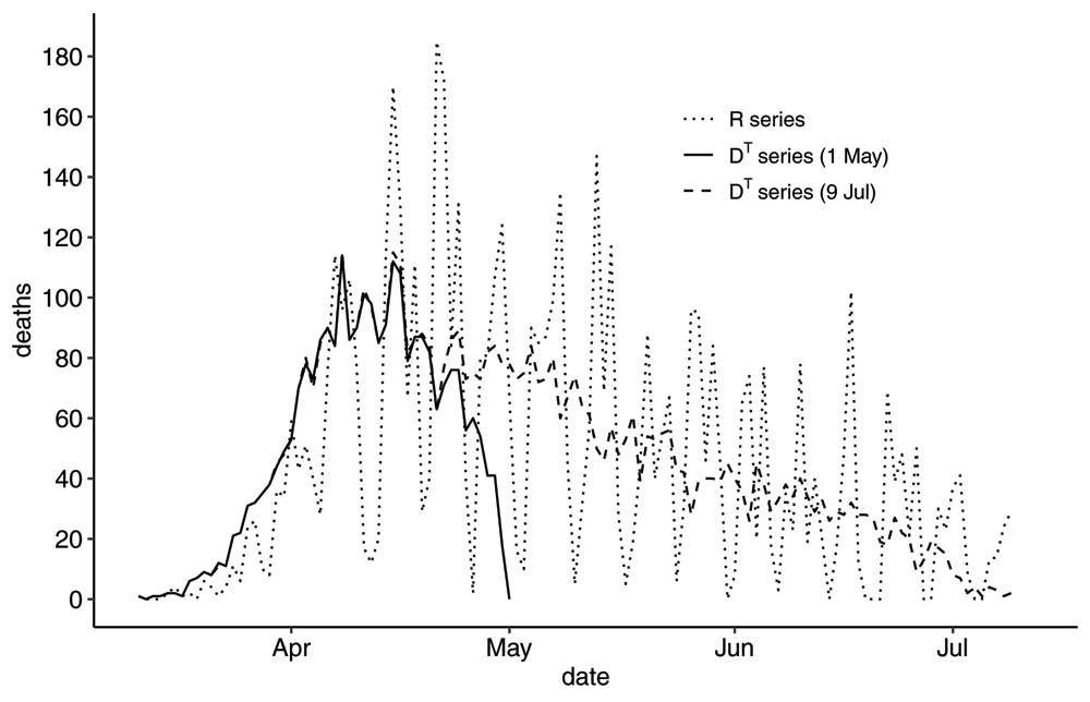
he R-series and the D^T-series as reported by Sweden on 2020-05-01 and on 2020-07-09. It is enough to plot just one R-series as it does not change retrospectively unlike the D^T-series, which is updated retrospectively every time it is reported.

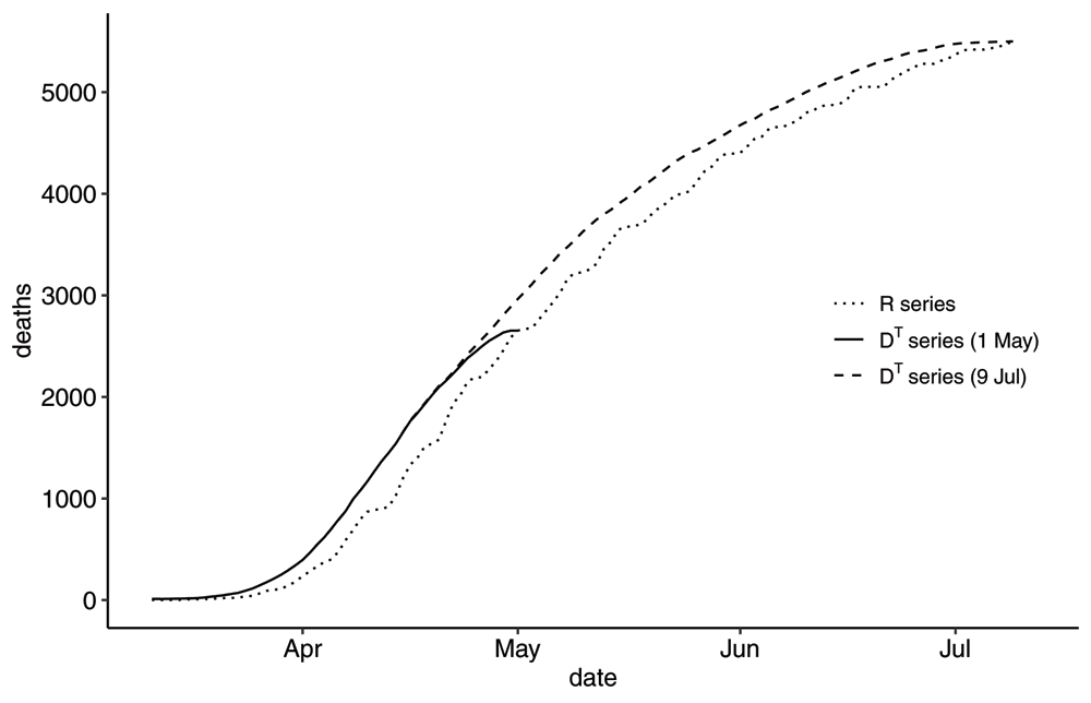
Figure 2. The cumulative deaths series.

The cumulative R-series and the cumulative D^T-series as reported by Sweden on 2020-05-01 and on 2020-07-09. Clearly, there is a delay in the R-series compared to the D^T-series. The cumulative number of deaths coincide for both series on the reporting day.

In addition to comparing the R-series and the D^T-series, we will say a few words about nowcasting, and introduce a naive method based on the characteristics of the reporting process.

Materials and methods

It turns out that there is a rather elegant mathematical framework for the two series in terms of matrix algebra. For the interested reader we have put all of that in the Appendix (see Extended data¹³). One of the key findings is equation (A16) which is the mathematical relationship between the R-series and the D^T-series which is worth repeating here. The relationship between r_t and $d_{e}^{T}$ is

r_{t} = \sum_{e = 0}^{T} ρ_{e}^{T} (t - e) d_{e}^{T} (4)

where $ρ_{e}^{T} (Δ)$ is the so-called forward-looking probability mass function (pmf) defined as the fraction of the deaths that happened on event date e and were reported exactly Δ days later. If there were underlying stochastic variables for when deaths happened and were reported, $ρ_{e}^{T} (Δ)$ would have the interpretation as an estimate of the conditional probability P(reporting date = e+Δ | event date = e). There is also a corresponding forward-looking cumulative distribution function (cdf) $ϕ_{e}^{T} (Δ)$ defined as the the fraction of the deaths that happened on event date e and were reported within Δ days.

The expression (4) makes intuitive sense. It says that the number of deaths reported on day t, is the weighted sum of deaths happening on previous event days. The contribution from each event day e is the total number of deaths that day $d_{e}^{T}$ times the probability that those deaths will be reported exactly t–e days later.

Now, typically the reporting process does not change that much over time, in which case one may want to find the average cumulative distribution function and the average probability mass function. See expression (A15) in the Appendix (see Extended data¹³) for how this is done. Also see the equation (A20) in the Appendix (see Extended data¹³) for the inverse of (4), i.e. $d_{e}^{T}$ as a function of r_t.

Equation (4) is interesting from another perspective. It is the defining expression of a linear time-dependent filter, where in-signal x(t) is modulated by a time dependent filter function f (τ, t, –τ) resulting in an out-signal y(t)

y (t) = \int_{0}^{\infty} f (τ, t - τ) x (τ) d τ (5)

In mathematical terms, the expression (5) is a so-called convolution of the true signal and the time-dependent filter. Filters are used in many areas including epidemiology, although its main application is in signal processing. Interestingly, studies of time-dependent filters relevant to this paper can be found in geology, e.g. in^14,15. The main insight here is that the practice of reporting daily deaths, the R-series, as is standard procedure, should be viewed as a time-dependent filter modulating the event-based curve. The reporting series R is distinct from the true death curve, even if it in most practical applications comes very close. Below we will highlight some circumstances where this difference can be important.

Nowcasting of the D^T-series

As can be seen in Figure 1, the D^T-series typically descends to a value close to zero on the reporting day T. This is because few deaths will be reported on the same day they actually happened. Many deaths have happened but are still being processed in the reporting system and will be reported at a later date. This means that for a time period prior to the reporting time, the D^T-series will underestimate the actual number of deaths on those days. Ideally, one would like to know the final number of deaths on any particular event date e before the reporting date T, i.e. finding the M series for t < T. This is the problem of nowcasting. Several groups have devised algorithms to estimate the M-series for t < T, see^16–22. In the Appendix (see Extended data¹³) we derive a very simple expression for the M-series, i.e. for m_e = $d_{e}^{\infty}$ , which is

m_{e} = d_{e}^{\infty} = d_{e}^{T} / ϕ_{e}^{\infty} (T - e) (6)

Intuitively this expression makes sense. It says that one could get the final number of deaths on an event day e by dividing the number of deaths on that day that have been reported so far (i.e. $d_{e}^{T}$ ) by $ϕ_{e}^{\infty} (T - e)$ , which the fraction of the final number of deaths on day e reported within T–e days since day e. Of course, at time T we don’t know what the final cdf $ϕ_{e}^{\infty}$ will look like but by making the assumption that the reporting process will behave as it has done in the recent past, we will be able to compute simple nowcasts below. The drawback of this method is that it does not work when $d_{e}^{T} = 0$ , but as we will see it can still be quite useful.

Source data and data processing

The computations in this paper have been based on the fundamental data set $d_{e t}^{T},$ which was constructed from downloading the D^T-series daily from 2020-04-02 to 2020-07-09. Data processing was done in R-studio (v1.2.1335) using R version 3.6.0 (2019-04-26). An R-script including relevant R-packages has been made available. Further information can be found in the Data availability section¹³23.

Results

We will now apply the methods described above and, in the Appendix (see Extended data¹³), to analyze the relationship between the reporting series and the event-based series as reported by Sweden.

The Swedish reporting process for Covid-19 deaths

As we have argued, the reporting process is characterized by the two time-dependent distribution functions $ϕ_{e}^{T} (Δ)$ and $ρ_{e}^{T} (Δ)$ . In Figure 3 we have plotted the cumulative distribution functions for all event dates between 2020-04-02 and 2020-06-01, as well as the resulting mean cdf.

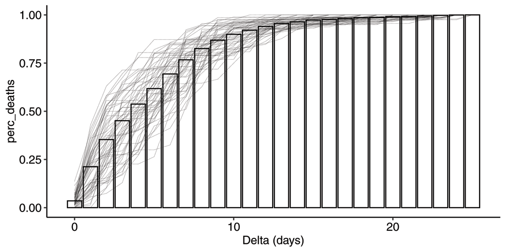
Figure 3. The cdfs for the Swedish reporting process of deaths.

Plot of all cdfs $ϕ_{e}^{T} (Δ)$ for event dates between 2020-04-02 and 2020-06-01. The bars represent the mean cdf which is time independent. The cdf $ϕ_{e}^{T} (Δ)$ is defined as the fraction of deaths on a particular event date e that will be reported within Δ days.

In Figure 4 we show the corresponding mean pmf $ρ_{e}^{T} (Δ)$ . The first observation is that there is a significant delay in the reporting process. The average delay can be computed using equation (A14) and is 5.2 days. By inspection of the cdf, we see that it takes on average 7 days to capture 75% of the deaths on a particular day, and about 10 days to capture 90% of the deaths.

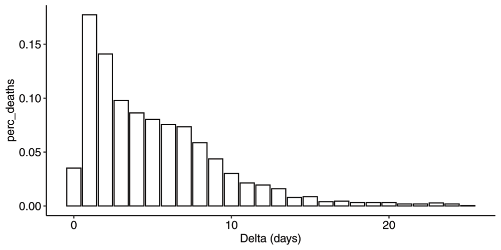
Figure 4. The mean pmf for the Swedish reporting process of deaths.

Plot of the mean probability mass function corresponding to the mean cdf across all event days between 2020-04-02 and 2020-06-01.

Furthermore, from inspection of the pmf in Figure 4, there seems to be a substructure to the reporting process. One can identify three sub-processes with different delays. Allow us to speculate that we have one reporting process for deaths in hospitals with an average delay of 1–2 days, one process for deaths in nursing homes with an average delay of 6–7 days and a third process that for some reason takes even longer, with an average delay of 11–12 days. One can imagine the pmf resulting from superposition of three distributions where the respective areas under the curve correspond to the fraction of deaths in those three settings respectively. Again, by inspection of the pmf, we estimate that roughly 3/8, 1/2 and 1/8 of the deaths happened in those three settings respectively. This is roughly in line with what has been reported by Sweden²⁴.

In order to better understand the weekly periodic pattern in the R-series, we have computed the average distributions for each weekday. The average cumulative distribution functions for each weekday is plotted in Figure 5. There is a flat portion of each curve representing the fact that deaths were essentially not reported on Sundays. For Saturdays the flat portion is between day 0 and day 1; for Fridays between day 1 and 2 etc. Sweden stopped reporting both the R and the D^T-series on weekends from 2020-06-20 onwards.

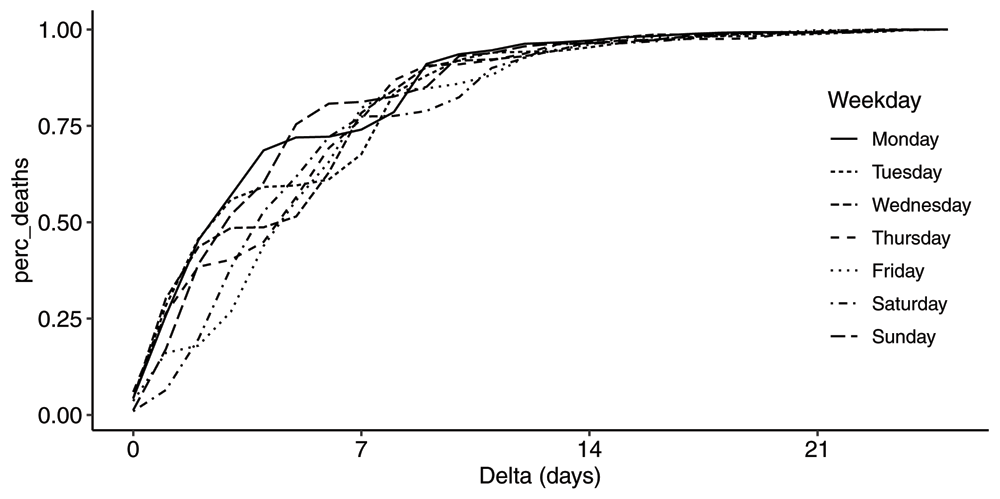
Figure 5. The average cdfs by weekday for the Swedish reporting process of deaths.

Plot of the average cdfs by weekday, for all event days between 2020-04-02 and 2020-06-01.

We also plot the pmfs in Figure 6. Given the simplicity of the mean distribution, the differences by weekday are a little surprising. It is a complex interplay between the three sub-processes mentioned previously and a significantly reduced reporting on Saturdays and Sundays resulting in the "valley" on day 6 on Mondays moving one day to the left every day.

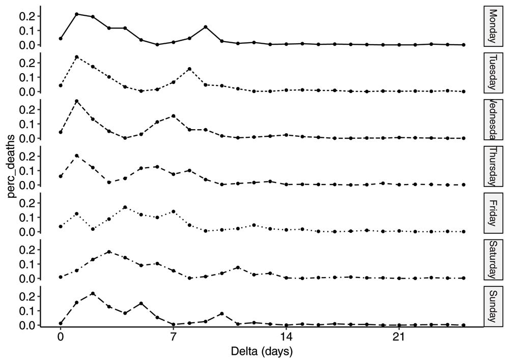
Figure 6. The average pmfs by weekday for the Swedish reporting process of deaths.

Plot of the average pmfs by weekday, for all event days between 2020-04-02 and 2020-06-01.

Next, in order to isolate the effect of the reporting process, we compute the effect of the Swedish reporting process on a hypothetical smooth bell shaped death curve, much like we have done for two simple examples in Figure A11 and Figure A12 in the Appendix (see Extended data¹³). The result can be seen in Figure 7.

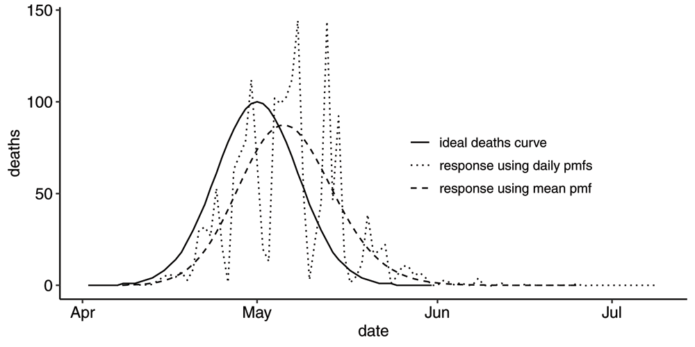
Figure 7. Application of the Swedish reporting process to a hypothetical death curve.

Plot of the Swedish reporting process applied to a hypothetical smooth bell-shaped actual deaths curve. The R-series resulting from application of the full time-dependent set of pmfs shows a response very similar to reported R-series. The R-series resulting from the application of the time-independent mean pmf produces a modified bell-shaped R-series which is flatter and wider with a slightly different slope.

Again, the daily, time-dependent pmfs produce a highly variable output just like the observed reporting series. Contrasting this output to the output one gets using the mean time-independent pmf, we conclude that the periodic pattern in the reporting series has its origin in characteristics of the reporting process rather than in the characteristics of the actual deaths curve. Although this is perhaps not very surprising, the amplitude of the periodic pattern is surprising. Relatively small differences in the reporting processes from one weekday to the next results in these wild swings in the reported daily deaths. Is there an opportunity to give guidance to the countries for how to reduce these resulting swings? We also note that the Swedish reporting process modifies the shape of the hypothetical death curve in three ways, just like the hypothetical cases in the Appendix (see Extended data¹³). First, there is a clear time shift. Second, the peak is lower. Third, the slope is flatter, both as deaths increase and decrease.

Smoothing of the Swedish R-series

As we have seen, the Swedish R-series is very variable. Hence, when using the R-series as model input one may have to do some pre-processing. If used in a time dependent model together with case incidence or prevalence (e.g. in an SIR model) one may have to adjust for the reporting delay, since the reporting of cases normally is quicker than the reporting of deaths. The average reporting delay for cases in Sweden is approximately 1–2 days.

Additionally, if initial conditions need to be specified for the magnitude as well as the slope of the death curve, some kind of smoothing of the R-series is appropriate. The question then arises, what is a good smoothing of the R-series? Since the R-series is not the same as the D^T-series, what should a good smoothing of the R-series look like? The example in the previous section gives us a clue. Based on the graphs plotted in Figure 7, a measure of how good a smoothing is to see how closely it matches the "transformed" D^T-series, i.e. the series one would obtain by applying a "smoothed reporting process" to the event based series, i.e. using the time-independent mean pmf rather than the time-dependent pmfs. In addition, a good smoothing should have the same area under the curve as the R-series. Unfortunately, neither the D^T-series, nor the mean pmf are available to the modelers.

One model that relies on the shape of the death curve is the model developed by the Institute of Health Metrics and Evaluations (IHME) at University of Washington²⁵. In Figure 8 we have plotted the Swedish R-series as reported on 2020-06-03 well as the smoothing of the R-series by IHME modelers in the 2020-06-05 update of their model²⁶. We have also plotted the transformed D^T-series one obtains by filtering the D^T series using the mean pmf.

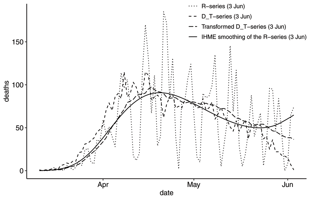
Figure 8. Smoothing of the Swedish R-series.

Plot showing the IHME smoothing of the R-series on 2020-06-03 in comparison with the Transformed D^T-series using the mean pmf. Note there is an uptick in the R-series just before the reporting date, which may have influenced the smoothing. Also note that the Transformed D^T-series has a slightly lower peak, a significant delay and a lesser slope than the D^T-series.

At this particular instance the IHME modelers were unfortunate to produce a smoothing that drastically changed the outcome of the model and we can see that it deviates significantly from the transformed D^T-series. This IHME smoothing preserved the number of deaths. For reference, the 2020-06-05 update of the model estimated 8357 (7046, 10386) number of deaths by 2020-08-01. A previous update on 2020-05-29, with a different smoothing, estimated 5254 (4688, 6420) number of deaths. In their next update of the model on 2020-06-25, the smoothing is very similar to the transformed D^T-series.

Please note that by only using the smoothed R-series as input, one does not compensate for the delay in the reporting process, nor for the change in shape of the curve. This means for the total number of deaths, as well as the rise (or decline) in number of deaths is underestimated.

Nowcasting of the Swedish D^T-series

Turning our attention to the D^T-series, we were curious to see how a state of the art nowcasting algorithm would perform in the presence of the strong weekly patterns in the Swedish time-dependent reporting process. We have therefore compared a "naive" approximation of the nowcasting formula (6) with the nowcasting algorithm developed by a group at Harvard¹⁷. We wanted to use both a time independent and a time-dependent approximation and used the following two naive approximations

ϕ_{e}^{\infty} (Δ) \approx ϕ_{21 - 34}^{\infty} (Δ) (Mean nowcast) (7)

ϕ_{e}^{\infty} (Δ) \approx \frac{1}{2} [ϕ_{e - 21}^{\infty} (Δ) + ϕ_{e - 28}^{\infty} (Δ)] (Weekday forecast) (8)

where $ϕ_{21 - 34}^{T} (Δ)$ is the mean cdf computed as an average of the 14 cdfs for the event days 21–34 days before the reporting time T. Note that we have to go 21 days back in order to have the cdf defined for Δ between 0 and 21 days. We deliberately chose a multiple of 7 to match with the correct weekday. Starting on Sunday 2020-05-10, we have plotted 7 nowcasts of the D^T-series. The first graphs are shown in Figure 9 and the following six in Figure 10.

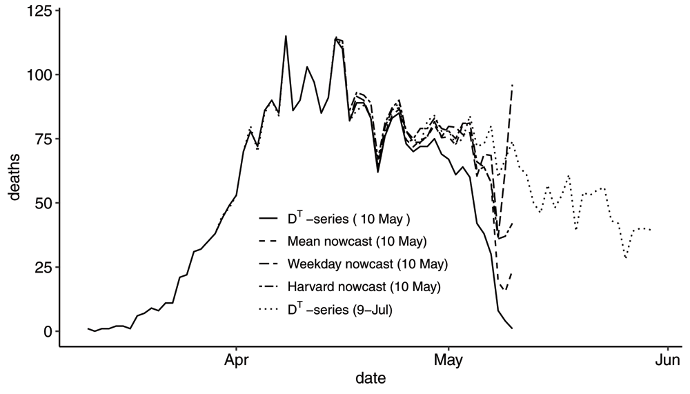
Figure 9. Nowcasts of the Swedish D^T-series, initial day.

Graph showing the D^T-series, the Mean nowcast, the Weekday nowcast and the Harvard nowcast of the D^T-series on the reporting day 2020-05-10. The D^T-series as of 2020-07-09 serves as the true M-series. On this reporting day, the three nowcasts are quite different for the two days prior to the reporting date.

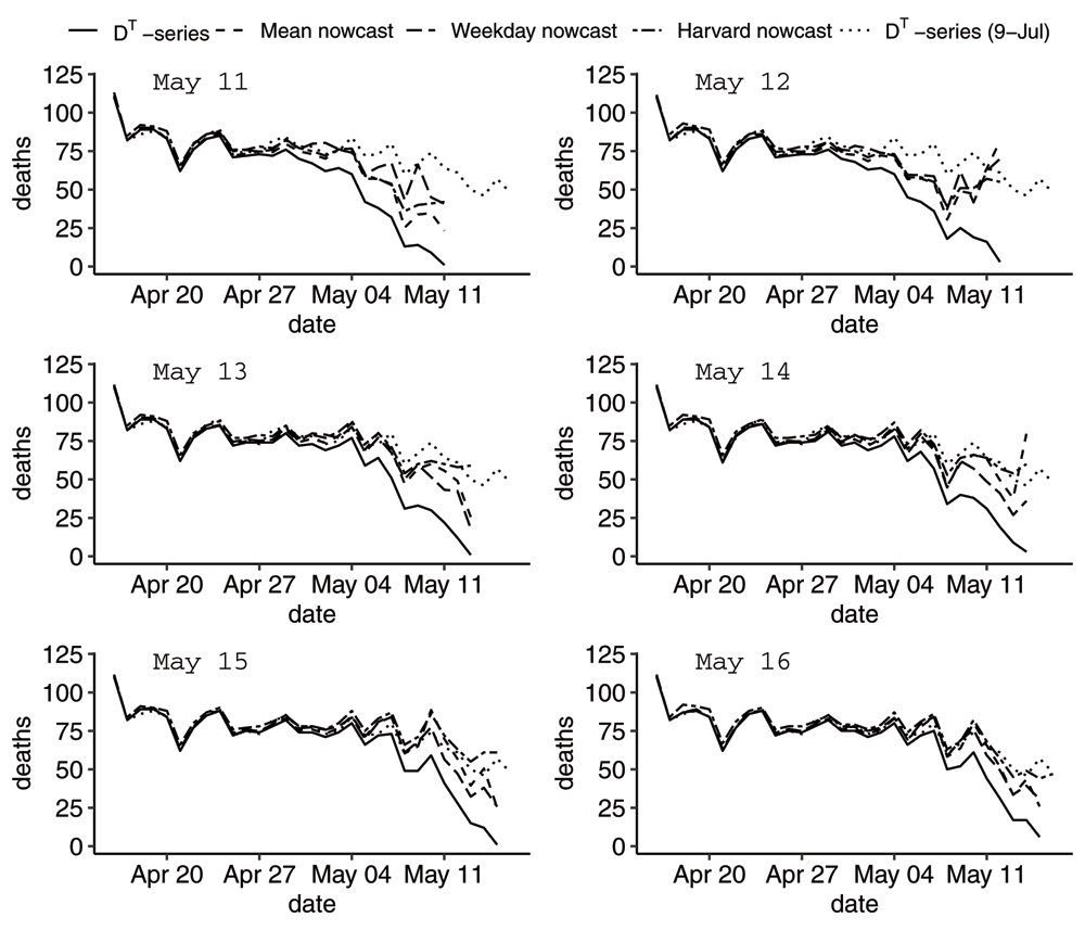
Figure 10. Nowcasts of the Swedish D^T-series, subsequent days.

Graph showing the zoomed-in D^T-series, the Mean nowcast, the Weekday nowcast and the Harvard nowcast of the D^T-series on reporting days between 2020-05-11 and 2020-05-16. The D^T-series as of 2020-07-09 serves as the true M-series. Although the Harvard nowcast is better, the naive nowcasts can be useful.

Generally, the Harvard nowcast algorithm performs better, but since also the Harvard nowcast fluctuates, it would be interesting to see if there are improvements that can be made by taking the weekly pattern better into account. It should be noted that we have used default settings for the Harvard nowcast. Furthermore, one can likely improve upon the approximations (7) and (8) but nowcasting is not the focus of this paper. The takeaway message here is that there are good nowcast methods available to analysts if they have access to the fundamental data set $d_{e t}^{T}$ and if they are interested in using the best possible input in their analyses.

Conclusion

By viewing the R-series and the D^T-series as two aspects of the same underlying data set, we conclude that the R-series is the result of a reporting process that "filters" the event based series, the D^T-series, see Equation (4). In many cases this does not result in a significant difference between the two series. However, it turns out that the Swedish reporting process for Covid-19 deaths happens to generate a R-series that looks quite different from the D^T-series. The R-series is wildly varying in time, which makes it hard to see trends and use as model input.

To remedy this for the Swedish R-series, smoothing of the curve is appropriate. Unfortunately, it is hard to know what constitutes a good smoothing, unless you have access to the D^T-series. However, three factors are worth paying close attention to. First, most reporting processes have a built-in delay, leading to a corresponding shift in time between the R-series and the D^T-series. Second, if the delay is significant, the shape of the curve will also be affected. The peak will be lower, and the slope of the smooth R-series will be less than the slope of the D^T-series. This may result in an estimate of number of deaths that is an under-estimate during times of increasing daily deaths counts, and an over-estimate during times of decreasing death counts. Finally, if the slope of the deaths curve just before the reporting time is of importance, one should note that the perfectly smooth R-series will to some degree reflect the slope of the D^T-series and drop off just before the reporting time. Getting the slope right based on the R-series can therefore be a very hard problem, as we have seen in a real world case shown in Figure 8. It is worth noting that smoothing of the R-series by applying a 7- or 14-day rolling average, which has been very common when reporting Covid-19 deaths, might be a good idea but it suffers from the same short comings as mentioned above. It adds another four (alt. eight) days of delay, dampens the peaks, and additionally flattens the slope of the death curve.

So, what is the best method? In cases where the there is a significant difference between the R-series and the D^T-series, it is probably not very controversial to be of the opinion that one should use the D^T-series. However, one then faces the problem of a D^T-series that drops off to zero close to the reporting date, see Figure 1, and one is forced to use a nowcasting method to compensate for this drop-off. As we have seen in Figure 9 and Figure 10, the nowcasting series are not perfect and do fluctuate when applied to the Swedish data set. Nevertheless, whereas the change in shape of the R-series from one day to another can be significant, the shape of D^T-series never changes that much since it distributes the new deaths over many event dates. This is the main reason why using the D^T-series with nowcasting is preferable to using the R-series with smoothing, shifting and potentially compensating for a difference in shape.

Coming back to the Swedish situation, back in May it was not a trivial task to interpret the death curve and seeing the trend if you only had access to the R-series. However, having access to the D^T-series and a nowcasting algorithm did give you confidence that the number of deaths were indeed declining. Of course, access to data for hospitalizations, ICU occupancy and case incidence gives a more complete picture and help interpret the situation. Nevertheless, it would be welcome if more countries made the D^T-series available.

Data availability

Underlying data

The primary data set analyzed in this paper was constructed by downloading the D^T-series daily from the Public Health Agency of Sweden⁷ between 2020-04-02 and 2020-07-09. The data is publicly available and is considered public domain data.

Zenodo: On the use of real-time mortality data in modelling and analysis during an epidemic outbreak – underlying data

https://doi.org/10.5281/zenodo.3992345²³.

This project contains the following underlying data:

FHM_Covid_Download.zip. (Zip-archive of raw downloaded files with Swedish deaths data.)
swedish_covid_deaths_data.csv. (Swedish deaths data collated from the raw data files in a .csv format.)
swedish_covid_deaths_data.xlsx. (Swedish deaths data collated from the raw data files in a .xlsx format.)

Data are available under the terms of the Creative Commons Zero "No rights reserved" data waiver (CC0 1.0 Public domain dedication).

In the article we also discuss and plot data generated by Institute of Health Metrics and Evaluation²⁶ in the 2020-06-05 update of their model. The terms and conditions can be found or their website and states for non-commercial users: “Data made available for download on IHME Websites can be used, shared, modified or built upon by non-commercial users via the Creative Commons Attribution-NonCommercial 4.0 International License (https://creativecommons.org/licenses/by-nc/4.0/)”.

Extended data

The Appendix to this article as well as the R-code to generate the graphs and the nowcasts are available as extended data.

Zenodo: On the use of real-time mortality data in modelling and analysis during an epidemic outbreak – extended data.

http://doi.org/10.5281/zenodo.4005244¹³.

This project contains the following extended data:

Liljenberg2020_OGR_Appendix.pdf (Appendix to the main article)
swedish_covid_deaths_OGR.R. (R-script to generate graphs and nowcasts in the paper.)
MDAR author checklist.pdf (Completed MDAR reporting checklist)

Data are available under the terms of the Creative Commons Zero "No rights reserved" data waiver (CC0 1.0 Public domain dedication).

Acknowledgements

We would like to acknowledge Dr. Sarah McGough for assistance with the Harvard nowcasting r-package.

Faculty Opinions recommended

References

1. World Health Organization (WHO): Coronavirus Disease (COVID-19) Situation Reports. [Accessed: 01-Aug-2020]. Reference Source
2. Centers for Disease Control and Prevention (U.S.): CDC COVID Data Tracker. [Accessed: 01-Aug-2020].
3. European Centre for Disease Control: How ECDC collects and processes COVID-19 data. 2020. [Accessed: 05-Jul-2020]. Reference Source
4. Johns Hopkins University: COVID-19 Map - Coronavirus Resource Center. 2020. [Accessed: 01-Aug-2020]. Reference Source
5. Dong E, Du H, Gardner L: An interactive web-based dashboard to track COVID-19 in real time. Lancet Infect Dis. Lancet Publishing Group. 2020; 20(5): 533–534. PubMed Abstract | Publisher Full Text | Free Full Text
6. Our World in Data: Coronavirus Pandemic (COVID-19) - Statistics and Research. [Accessed: 01-Aug-2020]. Reference Source
7. Folkhälosmyndigheten (Public health agency of Sweden): Bekräftade fall i Sverige — Folkhälsomyndigheten. [Accessed: 10-Jul-2020]. Reference Source
8. Folkhälsomyndigheten (Public health agency of Sweden): Bekräftade fall i Sverige - daglig uppdatering. [Accessed: 05-Jul-2020]. Reference Source
9. Sveriges Television: The spread of the new coronavirus - SVT Nyheter. [Accessed: 05-Jul-2020]. Reference Source
10. Sciensano (Belgian Institute for Health): Epistat - COVID-19 Monitoring. 2020. [Accessed: 18-Aug-2020]. Reference Source
11. National Health Service: Statistics » COVID-19 Daily Deaths. [Accessed: 10-Jul-2020]]. Reference Source
12. GOV.UK: Coronavirus (COVID-19) in the UK. [Accessed: 05-Jul-2020]. Reference Source
13. Liljenberg P: On the use of real-time mortality data in modelling and analysis during an epidemic outbreak - extended data [Data set]. Zenodo. 2020. http://www.doi.org/10.5281/zenodo.4005244
14. Margrave GF: Theory of nonstationary linear filtering in the Fourier domain with application to time‐variant filtering. GEOPHYSICS. 1998; 63(1): 244–259. Publisher Full Text
15. Clarke GKC: Time-varying deconvolution filters. GEOPHYSICS. 1968; 33(6): 936–944. Publisher Full Text
16. Salmon M, Schumacher D, Stark K, et al.: Bayesian outbreak detection in the presence of reporting delays. Biom J. 2015; 57(6): 1051–1067. PubMed Abstract | Publisher Full Text
17. McGough SF, Johansson MA, Lipsitch M, et al.: Nowcasting by Bayesian Smoothing: A flexible, generalizable model for real-time epidemic tracking. PLOS Comput Biol. 2020; 16(4): e1007735. PubMed Abstract | Publisher Full Text | Free Full Text
18. Rotejanaprasert C, Ekapirat N, Areechokchai D, et al.: Bayesian spatiotemporal modeling with sliding windows to correct reporting delays for real-time dengue surveillance in Thailand. Int J Health Geogr. 2020; 19(1): 4. PubMed Abstract | Publisher Full Text | Free Full Text
19. Wu JT, Leung K, Leung GM: Nowcasting and forecasting the potential domestic and international spread of the 2019-nCoV outbreak originating in Wuhan, China: a modelling study. Lancet. 2020; 395(10225): 689–697. PubMed Abstract | Publisher Full Text | Free Full Text
20. Arslan S, Ozdemir MY, Ucar A: Nowcasting and Forecasting the Spread of COVID-19 and Healthcare Demand In Turkey, A Modelling Study. medRxiv. 2020. Publisher Full Text
21. Science Media Centre: Nowcasting and forecasting COVID-19 data. [Accessed: 01-Aug-2020]. Reference Source
22. Bird S, Nielsen B: Now-casting of Covid-19 deaths in English hospitals. [Accessed: 21-Jun-2020]. Reference Source
23. Liljenberg P: On the use of real-time mortality data in modelling and analysis during an epidemic outbreak - underlying data [Data set]. Zenodo. 2020. http://www.doi.org/10.5281/zenodo.3992345
24. Socialstyrelsen: Statistik om covid-19 bland äldre efter boendeform - Socialstyrelsen. [Accessed: 11-Jul-2020]. Reference Source
25. IHME COVID-19 health service utilization forecasting team, Murray CJL: Forecasting the impact of the first wave of the COVID-19 pandemic on hospital demand and deaths for the USA and European Economic Area countries. medRxiv. 2020. Publisher Full Text
26. IHME COVID-19 health service utilization forecasting team, Murray CJL: COVID-19 estimate downloads | Institute for Health Metrics and Evaluation. [Accessed: 10-Jul-2020]. Reference Source

Comments on this article Comments (0)

Version 1

VERSION 1 PUBLISHED 11 Sep 2020

Author details Author details

Bill & Melinda Gates Foundation, Seattle, WA, USA

Per Liljenberg
Roles: Conceptualization, Data Curation, Formal Analysis, Investigation, Methodology, Project Administration, Resources, Software, Supervision, Validation, Visualization, Writing – Original Draft Preparation, Writing – Review & Editing

Competing interests

No competing interests were disclosed.

Grant information

The author is an employee of the Bill & Melinda Gates Foundation.

Article Versions (1)

version 1

Published: 11 Sep 2020, 4:128

https://doi.org/10.12688/gatesopenres.13180.1

Copyright

© 2020 Liljenberg P. This is an open access article distributed under the terms of the Creative Commons Attribution License, which permits unrestricted use, distribution, and reproduction in any medium, provided the original work is properly cited.

Download

Export To

metrics

	Views	Downloads
Gates Open Research	-	-
PubMed Central Data from PMC are received and updated monthly.	-	-

Citations

0

SEE MORE DETAILS

CITE

how to cite this article

Liljenberg P. On the use of real-time reported mortality data in modelling and analysis during an epidemic outbreak [version 1; peer review: 2 approved with reservations]. Gates Open Res 2020, 4:128 (https://doi.org/10.12688/gatesopenres.13180.1)

NOTE: If applicable, it is important to ensure the information in square brackets after the title is included in all citations of this article.

track

receive updates on this article

Track an article to receive email alerts on any updates to this article.

Open Peer Review

Version 1

VERSION 1

PUBLISHED 11 Sep 2020

Views

12

Reviewer Report 29 Jan 2021

Shaun Truelove, Department of International Health, Johns Hopkins Bloomberg School of Public Health, Baltimore, MD, USA

Approved with Reservations

https://doi.org/10.21956/gatesopenres.14380.r30074

This paper presents an interesting examination of how aggregate death reporting can misrepresent the true mortality curve during the COVID-19 pandemic. Using case data, which captures the true dates of when deaths happened, not just when they were reported, the ... Continue reading

This paper presents an interesting examination of how aggregate death reporting can misrepresent the true mortality curve during the COVID-19 pandemic. Using case data, which captures the true dates of when deaths happened, not just when they were reported, the author developed a mathematical framework for compare the sources of deaths. Through this framework, the author goes on to compare the now-casting with their framework with those of IHME and Harvard.

While the methods are sound, the structure of this manuscript was unconventional, making it somewhat challenging to follow. The author provided only limited background information, and motivation for this work was not overtly clear to the reader. I would like to see more background provided about why we care about these differences in deaths reporting.

The methods and results were similarly lacking in structure. I was not completely clear what the authors did in terms of methods, particularly with respect to the now-casting, and much of the results are presented as a conversational commentary, rather than scientific findings. It would have been good to seen a quantified impact of using the R-series versus the D-series.

Finally, while I believe this work provides novel findings, I believe these findings could be more clearly presented and emphasized, particularly in terms of how the public should be interpreting model results, and how researchers should be accounting for these. Additionally, the author did not discuss limitations of this work or reliability of the data being used. While the "D-series" is ideal, it is often only a subset of individuals across a country.

Is the work clearly and accurately presented and does it cite the current literature?

Partly
Is the study design appropriate and is the work technically sound?

Partly
Are sufficient details of methods and analysis provided to allow replication by others?

Yes
If applicable, is the statistical analysis and its interpretation appropriate?

Yes
Are all the source data underlying the results available to ensure full reproducibility?

Yes
Are the conclusions drawn adequately supported by the results?

Yes

Competing Interests: No competing interests were disclosed.

Reviewer Expertise: infectious disease epidemiology and modeling, statistics, COVID-19, vaccination

I confirm that I have read this submission and believe that I have an appropriate level of expertise to confirm that it is of an acceptable scientific standard, however I have significant reservations, as outlined above.

CITE

Report a concern

Respond or Comment

Views

28

Reviewer Report 18 Nov 2020

Subhas Khajanchi, Department of Mathematics, Presidency University, Kolkata, West Bengal, India

Approved with Reservations

https://doi.org/10.21956/gatesopenres.14380.r29961

The COVID-19 pandemic has already spread throughout the world and the people are aware about the diseases and they are using precautions about the pandemic. Still, COVID-19 is spreading very quickly. Some countries like Spain, Australia, Serbia, China, etc. have ... Continue reading

The COVID-19 pandemic has already spread throughout the world and the people are aware about the diseases and they are using precautions about the pandemic. Still, COVID-19 is spreading very quickly. Some countries like Spain, Australia, Serbia, China, etc. have started a second wave of COVID-19. To stop the spread of the disease, a vaccine is needed. In absence of the vaccine people must have maintained social distancing. In order to maintain the social distancing, one must obey the modeling rule.

The introduction needs to be improved by incorporating some recent references of COVID-19 pandemic. To do so, I suggest some modeling work to be included in the references such as: Sakar et al. (2020)¹, Khajanchi & Sakar (2020)², and Samui et al. (2020)³.

In this context, an important factor must be included in this study, that is, the impact of the effect of media. How the COVID-19 dynamics been changed due to incorporation of the media related awareness like use of face masks, non-pharmaceutical interventions, hand sanitization, etc. The author must include the manuscript Khajanchi et al. (2020)⁴ to study the effect of media.

Is there any experimental data to validate the mathematical model? The authors at least describe the basic reproduction number R₀ and its impact on COVID-19 pandemic in India. The basic reproduction number R₀ is one of the most crucial quantities in infectious diseases, as R₀ measures how contagious a disease is. For R₀ < 1, the disease is expected to stop spreading, but for R₀ = 1 an infected individual can infect on an average 1 person, that is, the spread of the disease is stable. The disease can spread and become epidemic if R₀ must be greater than 1⁵.

Some references contain errors and inconsistent formatting. It is difficult to give credit to research if even elementary aspects of the work are not error free. This should be corrected with care and love to detail.

The manuscript is comprehensive, and I have enjoyed learning about the presented results. I find that the manuscript is written with very poor language and the presentation is not good, and I am in principal in favor of indexing, although the following comments should nevertheless be accommodated in one major revision.

Is the work clearly and accurately presented and does it cite the current literature?

Partly
Is the study design appropriate and is the work technically sound?

Partly
Are sufficient details of methods and analysis provided to allow replication by others?

Yes
If applicable, is the statistical analysis and its interpretation appropriate?

Partly
Are all the source data underlying the results available to ensure full reproducibility?

Partly
Are the conclusions drawn adequately supported by the results?

Partly

References

1. Sarkar K, Khajanchi S, Nieto JJ: Modeling and forecasting the COVID-19 pandemic in India.Chaos Solitons Fractals. 2020; 139: 110049 PubMed Abstract | Publisher Full Text
2. Khajanchi S, Sarkar K: Forecasting the daily and cumulative number of cases for the COVID-19 pandemic in India.Chaos. 2020; 30 (7): 071101 PubMed Abstract | Publisher Full Text
3. Samui P, Mondal J, Khajanchi S: A mathematical model for COVID-19 transmission dynamics with a case study of India.Chaos Solitons Fractals. 2020; 140: 110173 PubMed Abstract | Publisher Full Text
4. Khajanchi S, Sarkar K, Mondal J, Perc M: Dynamics of the COVID-19 pandemic in India. 2020. Publisher Full Text
5. Khajanchi S, Bera S, Roy T: Mathematical analysis of the global dynamics of a HTLV-I infection model, considering the role of cytotoxic T-lymphocytes. Mathematics and Computers in Simulation. 2021; 180: 354-378 Publisher Full Text

Competing Interests: No competing interests were disclosed.

Reviewer Expertise: Infectious diseases, Ecological systems, Tumor-immune interactions.

I confirm that I have read this submission and believe that I have an appropriate level of expertise to confirm that it is of an acceptable scientific standard, however I have significant reservations, as outlined above.

CITE

Report a concern

Respond or Comment

Comments on this article Comments (0)

Version 1

VERSION 1 PUBLISHED 11 Sep 2020

Open Peer Review

Reviewer Status

Reviewer Reports

	Invited Reviewers
	1	2
Version 1 11 Sep 20	read	read

Subhas Khajanchi, Presidency University, Kolkata, India
Shaun Truelove, Johns Hopkins Bloomberg School of Public Health, Baltimore, USA

Comments on this article

All Comments(0)

Add a comment

Sign up for content alerts

Back to all reports

Reviewer Report

12 Views

29 Jan 2021 | for Version 1

Shaun Truelove, Department of International Health, Johns Hopkins Bloomberg School of Public Health, Baltimore, MD, USA

12 Views Cite this report Responses(0)

Approved With Reservations

This paper presents an interesting examination of how aggregate death reporting can misrepresent the true mortality curve during the COVID-19 pandemic. Using case data, which captures the true dates of when deaths happened, not just when they were reported, the author developed a mathematical framework for compare the sources of deaths. Through this framework, the author goes on to compare the now-casting with their framework with those of IHME and Harvard.

While the methods are sound, the structure of this manuscript was unconventional, making it somewhat challenging to follow. The author provided only limited background information, and motivation for this work was not overtly clear to the reader. I would like to see more background provided about why we care about these differences in deaths reporting.

The methods and results were similarly lacking in structure. I was not completely clear what the authors did in terms of methods, particularly with respect to the now-casting, and much of the results are presented as a conversational commentary, rather than scientific findings. It would have been good to seen a quantified impact of using the R-series versus the D-series.

Finally, while I believe this work provides novel findings, I believe these findings could be more clearly presented and emphasized, particularly in terms of how the public should be interpreting model results, and how researchers should be accounting for these. Additionally, the author did not discuss limitations of this work or reliability of the data being used. While the "D-series" is ideal, it is often only a subset of individuals across a country.

Is the work clearly and accurately presented and does it cite the current literature?

Partly
Is the study design appropriate and is the work technically sound?

Partly
Are sufficient details of methods and analysis provided to allow replication by others?

Yes
If applicable, is the statistical analysis and its interpretation appropriate?

Yes
Are all the source data underlying the results available to ensure full reproducibility?

Yes
Are the conclusions drawn adequately supported by the results?

Yes

Competing Interests

No competing interests were disclosed.

Reviewer Expertise

infectious disease epidemiology and modeling, statistics, COVID-19, vaccination

I confirm that I have read this submission and believe that I have an appropriate level of expertise to confirm that it is of an acceptable scientific standard, however I have significant reservations, as outlined above.

Respond to this report

Responses (0)

Back to all reports

Reviewer Report

28 Views

18 Nov 2020 | for Version 1

Subhas Khajanchi, Department of Mathematics, Presidency University, Kolkata, West Bengal, India

28 Views Cite this report Responses(0)

Approved With Reservations

The COVID-19 pandemic has already spread throughout the world and the people are aware about the diseases and they are using precautions about the pandemic. Still, COVID-19 is spreading very quickly. Some countries like Spain, Australia, Serbia, China, etc. have started a second wave of COVID-19. To stop the spread of the disease, a vaccine is needed. In absence of the vaccine people must have maintained social distancing. In order to maintain the social distancing, one must obey the modeling rule.

The introduction needs to be improved by incorporating some recent references of COVID-19 pandemic. To do so, I suggest some modeling work to be included in the references such as: Sakar et al. (2020)¹, Khajanchi & Sakar (2020)², and Samui et al. (2020)³.

In this context, an important factor must be included in this study, that is, the impact of the effect of media. How the COVID-19 dynamics been changed due to incorporation of the media related awareness like use of face masks, non-pharmaceutical interventions, hand sanitization, etc. The author must include the manuscript Khajanchi et al. (2020)⁴ to study the effect of media.

Is there any experimental data to validate the mathematical model? The authors at least describe the basic reproduction number R₀ and its impact on COVID-19 pandemic in India. The basic reproduction number R₀ is one of the most crucial quantities in infectious diseases, as R₀ measures how contagious a disease is. For R₀ < 1, the disease is expected to stop spreading, but for R₀ = 1 an infected individual can infect on an average 1 person, that is, the spread of the disease is stable. The disease can spread and become epidemic if R₀ must be greater than 1⁵.

Some references contain errors and inconsistent formatting. It is difficult to give credit to research if even elementary aspects of the work are not error free. This should be corrected with care and love to detail.

The manuscript is comprehensive, and I have enjoyed learning about the presented results. I find that the manuscript is written with very poor language and the presentation is not good, and I am in principal in favor of indexing, although the following comments should nevertheless be accommodated in one major revision.

Is the work clearly and accurately presented and does it cite the current literature?

Partly
Is the study design appropriate and is the work technically sound?

Partly
Are sufficient details of methods and analysis provided to allow replication by others?

Yes
If applicable, is the statistical analysis and its interpretation appropriate?

Partly
Are all the source data underlying the results available to ensure full reproducibility?

Partly
Are the conclusions drawn adequately supported by the results?

Partly

References

1. Sarkar K, Khajanchi S, Nieto JJ: Modeling and forecasting the COVID-19 pandemic in India.Chaos Solitons Fractals. 2020; 139: 110049 PubMed Abstract | Publisher Full Text
2. Khajanchi S, Sarkar K: Forecasting the daily and cumulative number of cases for the COVID-19 pandemic in India.Chaos. 2020; 30 (7): 071101 PubMed Abstract | Publisher Full Text
3. Samui P, Mondal J, Khajanchi S: A mathematical model for COVID-19 transmission dynamics with a case study of India.Chaos Solitons Fractals. 2020; 140: 110173 PubMed Abstract | Publisher Full Text
4. Khajanchi S, Sarkar K, Mondal J, Perc M: Dynamics of the COVID-19 pandemic in India. 2020. Publisher Full Text
5. Khajanchi S, Bera S, Roy T: Mathematical analysis of the global dynamics of a HTLV-I infection model, considering the role of cytotoxic T-lymphocytes. Mathematics and Computers in Simulation. 2021; 180: 354-378 Publisher Full Text

Competing Interests

No competing interests were disclosed.

Reviewer Expertise

Infectious diseases, Ecological systems, Tumor-immune interactions.

I confirm that I have read this submission and believe that I have an appropriate level of expertise to confirm that it is of an acceptable scientific standard, however I have significant reservations, as outlined above.

Respond to this report

Responses (0)

[1] 1. World Health Organization (WHO): Coronavirus Disease (COVID-19) Situation Reports. [Accessed: 01-Aug-2020]. Reference Source

[2] 2. Centers for Disease Control and Prevention (U.S.): CDC COVID Data Tracker. [Accessed: 01-Aug-2020].

[3] 3. European Centre for Disease Control: How ECDC collects and processes COVID-19 data. 2020. [Accessed: 05-Jul-2020]. Reference Source

[4] 4. Johns Hopkins University: COVID-19 Map - Coronavirus Resource Center. 2020. [Accessed: 01-Aug-2020]. Reference Source

[5] 5. Dong E, Du H, Gardner L: An interactive web-based dashboard to track COVID-19 in real time. Lancet Infect Dis. Lancet Publishing Group. 2020; 20(5): 533–534. PubMed Abstract | Publisher Full Text | Free Full Text

[6] 6. Our World in Data: Coronavirus Pandemic (COVID-19) - Statistics and Research. [Accessed: 01-Aug-2020]. Reference Source

[7] 7. Folkhälosmyndigheten (Public health agency of Sweden): Bekräftade fall i Sverige — Folkhälsomyndigheten. [Accessed: 10-Jul-2020]. Reference Source

[8] 8. Folkhälsomyndigheten (Public health agency of Sweden): Bekräftade fall i Sverige - daglig uppdatering. [Accessed: 05-Jul-2020]. Reference Source

[9] 9. Sveriges Television: The spread of the new coronavirus - SVT Nyheter. [Accessed: 05-Jul-2020]. Reference Source

[10] 10. Sciensano (Belgian Institute for Health): Epistat - COVID-19 Monitoring. 2020. [Accessed: 18-Aug-2020]. Reference Source

[11] 11. National Health Service: Statistics » COVID-19 Daily Deaths. [Accessed: 10-Jul-2020]]. Reference Source

[12] 12. GOV.UK: Coronavirus (COVID-19) in the UK. [Accessed: 05-Jul-2020]. Reference Source

[13] 13. Liljenberg P: On the use of real-time mortality data in modelling and analysis during an epidemic outbreak - extended data [Data set]. Zenodo. 2020. http://www.doi.org/10.5281/zenodo.4005244

[14] 14. Margrave GF: Theory of nonstationary linear filtering in the Fourier domain with application to time‐variant filtering. GEOPHYSICS. 1998; 63(1): 244–259. Publisher Full Text

[15] 15. Clarke GKC: Time-varying deconvolution filters. GEOPHYSICS. 1968; 33(6): 936–944. Publisher Full Text

[16] 16. Salmon M, Schumacher D, Stark K, et al.: Bayesian outbreak detection in the presence of reporting delays. Biom J. 2015; 57(6): 1051–1067. PubMed Abstract | Publisher Full Text

[17] 17. McGough SF, Johansson MA, Lipsitch M, et al.: Nowcasting by Bayesian Smoothing: A flexible, generalizable model for real-time epidemic tracking. PLOS Comput Biol. 2020; 16(4): e1007735. PubMed Abstract | Publisher Full Text | Free Full Text

[18] 18. Rotejanaprasert C, Ekapirat N, Areechokchai D, et al.: Bayesian spatiotemporal modeling with sliding windows to correct reporting delays for real-time dengue surveillance in Thailand. Int J Health Geogr. 2020; 19(1): 4. PubMed Abstract | Publisher Full Text | Free Full Text

[19] 19. Wu JT, Leung K, Leung GM: Nowcasting and forecasting the potential domestic and international spread of the 2019-nCoV outbreak originating in Wuhan, China: a modelling study. Lancet. 2020; 395(10225): 689–697. PubMed Abstract | Publisher Full Text | Free Full Text

[20] 20. Arslan S, Ozdemir MY, Ucar A: Nowcasting and Forecasting the Spread of COVID-19 and Healthcare Demand In Turkey, A Modelling Study. medRxiv. 2020. Publisher Full Text

[21] 21. Science Media Centre: Nowcasting and forecasting COVID-19 data. [Accessed: 01-Aug-2020]. Reference Source

[22] 22. Bird S, Nielsen B: Now-casting of Covid-19 deaths in English hospitals. [Accessed: 21-Jun-2020]. Reference Source

[23] 23. Liljenberg P: On the use of real-time mortality data in modelling and analysis during an epidemic outbreak - underlying data [Data set]. Zenodo. 2020. http://www.doi.org/10.5281/zenodo.3992345

[24] 24. Socialstyrelsen: Statistik om covid-19 bland äldre efter boendeform - Socialstyrelsen. [Accessed: 11-Jul-2020]. Reference Source

[25] 25. IHME COVID-19 health service utilization forecasting team, Murray CJL: Forecasting the impact of the first wave of the COVID-19 pandemic on hospital demand and deaths for the USA and European Economic Area countries. medRxiv. 2020. Publisher Full Text

[26] 26. IHME COVID-19 health service utilization forecasting team, Murray CJL: COVID-19 estimate downloads | Institute for Health Metrics and Evaluation. [Accessed: 10-Jul-2020]. Reference Source

On the use of real-time reported mortality data in modelling and analysis during an epidemic outbreak

Abstract

Keywords

Introduction

Figure 1. The daily deaths series.

Figure 2. The cumulative deaths series.

Materials and methods

Nowcasting of the D^T-series

Source data and data processing

Results

The Swedish reporting process for Covid-19 deaths

Figure 3. The cdfs for the Swedish reporting process of deaths.

Figure 4. The mean pmf for the Swedish reporting process of deaths.

Figure 5. The average cdfs by weekday for the Swedish reporting process of deaths.

Figure 6. The average pmfs by weekday for the Swedish reporting process of deaths.

Figure 7. Application of the Swedish reporting process to a hypothetical death curve.

Smoothing of the Swedish R-series

Figure 8. Smoothing of the Swedish R-series.

Nowcasting of the Swedish D^T-series

Figure 9. Nowcasts of the Swedish D^T-series, initial day.

Figure 10. Nowcasts of the Swedish D^T-series, subsequent days.

Conclusion

Data availability

Underlying data

Extended data

Acknowledgements

References

Comments on this article Comments (0)

Open Peer Review

Comments on this article Comments (0)

Open Peer Review

Reviewer Status

Reviewer Reports

Comments on this article

Are you a Gates-funded researcher?

Thank you!

On the use of real-time reported mortality data in modelling and analysis during an epidemic outbreak

Abstract

Keywords

Introduction

Figure 1. The daily deaths series.

Figure 2. The cumulative deaths series.

Materials and methods

Nowcasting of the DT-series

Source data and data processing

Results

The Swedish reporting process for Covid-19 deaths

Figure 3. The cdfs for the Swedish reporting process of deaths.

Figure 4. The mean pmf for the Swedish reporting process of deaths.

Figure 5. The average cdfs by weekday for the Swedish reporting process of deaths.

Figure 6. The average pmfs by weekday for the Swedish reporting process of deaths.

Figure 7. Application of the Swedish reporting process to a hypothetical death curve.

Smoothing of the Swedish R-series

Figure 8. Smoothing of the Swedish R-series.

Nowcasting of the Swedish DT-series

Figure 9. Nowcasts of the Swedish DT-series, initial day.

Figure 10. Nowcasts of the Swedish DT-series, subsequent days.

Conclusion

Data availability

Underlying data

Extended data

Acknowledgements

References

Comments on this article Comments (0)

Open Peer Review

Comments on this article Comments (0)

Open Peer Review

Reviewer Status

Reviewer Reports

Comments on this article

Competing Interests Policy

Stay Updated

Are you a Gates-funded researcher?

Thank you!

Nowcasting of the D^T-series

Nowcasting of the Swedish D^T-series

Figure 9. Nowcasts of the Swedish D^T-series, initial day.

Figure 10. Nowcasts of the Swedish D^T-series, subsequent days.