Keywords
Epidemiology, coinfection, serology, Bayesian statistics, repeated cross-sectional studies
Epidemiology, coinfection, serology, Bayesian statistics, repeated cross-sectional studies
Currently there are an estimated 38 million individuals infected with HIV1, while worldwide an estimated 71 million individuals are seropositive for HCV2. Estimates for HSV2 are even higher, at 400 million individuals3. Despite these high prevalences, estimating HIV, HCV and HSV2 incidence using current methods is challenging, and this difficulty is exacerbated by the initially asymptomatic nature of most of these infections. Incidence estimates are critical because they determine the current position of the leading edge of the epidemic and form part of WHO elimination targets4,5. In addition, at the population level, an accurate estimate of disease incidence allows countries to determine their future healthcare needs and assess the impact of prevention efforts.
There are a number of ways to estimate the population-level incidence of these diseases. The gold standard for incidence estimation is longitudinally-followed cohorts, measuring the rate of seroconversion by follow-up time. However, such longitudinal cohorts are expensive to maintain and suffer from selection bias and the Hawthorne effect6. Biomarker-based approaches also exist for measuring the incidence of HIV7,8, HCV9,10, and HSV211 via cross-sectional surveys. Although cross-sectional, biomarker-based methods have been applied to estimate HIV incidence in a number of settings12–14, the HCV and HSV2 biomarkers have not been validated as tools for estimating incidence at the population level. Therefore, cross-sectional studies of prevalence are still a standard tool for routine surveillance of these diseases15,16. These studies are still susceptible to a host of problems, including bias in the people surveyed, differential survival rates, and lack of information on anti-retroviral treatment status, but they are relatively simple to perform and provide an important insight despite studying a necessarily anonymous dataset.
Historically, the Johns Hopkins Hospital Emergency Department (JHH ED) has conducted serial identity-unlinked serosurveys to monitor the HIV epidemic among the marginalized inner-city populations of Baltimore, Maryland. These surveys demonstrated a high burden of HSV2, HIV and HCV, particularly among African Americans17–20. Previously they have been used to determine the care continuum among HIV infected individuals21, and also used to evaluate the recommended HCV testing guidelines22. These datasets include individual-level HIV, HCV, and HSV2 status, stratified by age, sex, and ethnicity. Though descriptive analyses are ongoing, a statistical analysis across multiple surveys to estimate incidence of multiple diseases, including coinfection rates, has not been undertaken. Where cross-sectional, age-stratified prevalence studies are available, there is a range of methodologies which could be used to analyse them to estimate incidence. These are often used to estimate HIV incidence23 and rarely used for HCV24. Statistical methodologies range from catalytic models, classically applied to measles and other childhood diseases, and more recently applied to malaria, to complex transmission models. Simpler models have the advantage that they are easy to parameterise and understand, but can be lacking more detailed transmission mechanisms. In contrast, complex models include more detailed mechanisms and correlations but are correspondingly difficult to parameterise and analyse.
It is rare for data to include multiple time points, and statistical techniques become more difficult to apply when there are many parameters and changing transmission rates in different groups. Considering co-infections only amplifies this problem, and so it is clear that to understand the interactions between diseases a new approach is needed. To this end we developed a novel differential equation model and fitted it to the data from three JHH ED serosurveys using Markov chain Monte Carlo methods. We jointly modelled incidence of infection and coinfection with HIV, HCV and HSV2 within age/gender cohorts and then fitted the model to the observed prevalence within a non-parametric Bayesian framework, allowing us to infer incidence rates that vary smoothly with time and age. We estimated the incidence of HIV, HCV and HSV2 on coinfections of these viruses among the JHH ED population before predicting the burden of disease and testing our model predictions against the fourth and final serosurvey.
At the adult JHH ED, identity-unlinked sero-surveys were conducted during six to eight-week periods in 2003, 2007, 2013 and 2016. These surveys are described in detail elsewhere21,25. Briefly, excess sera were collected and assigned a unique study ID while chart review data were recorded in real-time. All laboratory testing was done after the collection period when the linked patient identifiers were removed from the dataset. Patient consent was waived by the ethical review board. This study was approved by the Johns Hopkins School of Medicine Institutional Review Board (IRB00083646, CIR00016268) and conducted by the ethical standards of the Helsinki Declaration of the World Medical Association. In the current analysis the authors had access only to anonymized data consisting of the test outcomes, sex, race (coded as black, white or other), age category (yearly from 18 to 89, and over 89) alongside the year the test was performed. The analysis excludes multiple results per unique subject, those < 18 years of age and individuals that did not self-identify as black or white, male or female. The reason for this limitation is due to sample size limitations. We also excluded 31 patients with incomplete data for one or more tests. Prevalence summaries of the data, showing the changing age-profile of infection, are provided in Figure 1, and aggregated data is shown in Table 2.
In order to accurately model the movement of individuals through the various infection (and co-infection) classes, we need to know the excess mortality due to infection with HCV or HIV. HIV-specific mortality rates are taken from 26, a study estimating the age-stratified mortality of HIV positive individuals on antiretroviral therapy (ART). These rates may underestimate the excess mortality in our population since: the rates are not race-stratified; and the study population are all on ART. Conversely, these rates may overestimate mortality since: individuals on ART are unlikely to be recent infections; the study includes individuals with HCV; and the rates are not described relative to the background death rate. Table 1 gives the age- and year-specific mortality rates taken from 26. We assumed that the mortality rates remained constant after 2008.
| Data period | Age group | Mortality rate per 1000 person years |
|---|---|---|
| 2003–2005 | 20–34 | 10.7 |
| 2003–2005 | 35–44 | 19.7 |
| 2003–2005 | 45–54 | 26 |
| 2003–2005 | 55+ | 30.8 |
| 2006–2008 | 20–34 | 11 |
| 2006–2008 | 35–44 | 12.5 |
| 2006–2008 | 45–54 | 18.1 |
| 2006–2008 | 55+ | 27.4 |
| Serological status | Black female | Black male | White female | White male | Other (excluded) |
|---|---|---|---|---|---|
| 000 - Sero-negative | 926 | 1034 | 884 | 929 | 430 |
| 001 - HSV2 | 2236 | 903 | 408 | 210 | 155 |
| 010 - HIV | 13 | 42 | 2 | 15 | 23 |
| 011 - HIV+HSV2 | 134 | 112 | 5 | 16 | 28 |
| 100 - HCV | 53 | 241 | 39 | 143 | 2 |
| 101 - HCV+HSV2 | 322 | 352 | 96 | 82 | 8 |
| 110 - HCV+HIV | 4 | 67 | 0 | 7 | 4 |
| 111 - HCV+HIV+HSV2 | 18 | 169 | 14 | 14 | 4 |
| Total | 3806 | 2920 | 1448 | 1416 | 685* |
HCV-specific mortality rates were obtained from Mahajan et al., a cohort-study of HCV- infected patients which reports an annual mortality rate of 12.854% in the cohort, compared with 1.046% in the general population27. However to be included in the cohort, patients must be aware of their HCV status, which is not the case for the JHH ER data. Denniston et al. report that 50.3% of people detected with HCV were unaware they were infected28. We assumed that infected individuals needed to be aware to be included in the cohort described in Mahajan et al. and, since patients that are aware are more likely to have experienced symptoms, we assume that unaware individuals experienced a death rate similar to the general population. This results in a HCV mortality rate of 5.868% annual excess death rate. Finally Thomas et al. find that end-stage liver disease is 3.67 times more likely in those over 38 years of age29, and so we reduce the death rate from 5.868% for over 37s to 1.6% for under 38s.
We developed a novel cohort model (illustrated in Figure 2), in which individuals are born with no infection, and then, over their lifetime may acquire each of the three infections, in any order. Each vertex of the cube in Figure 2 represents a state an individual may be in. Each state is denoted by three digits, giving the status of each different disease (0 if uninfected with that disease and 1 if infected). The digits are given in the order: HCV, HIV and HSV2 so that, for example, 101 is the state of being infected with HCV and HSV2 and uninfected with HIV. We use this notation to write down a system of eight ordinary differential equations (ODEs), tracking the proportion of the population in each state over time. We divide the population into “cohorts” of individuals of similar ages and for each cohort we use the same eight ODEs, but allow the parameters (the λ’s and θ’s) to be different for different cohorts. Each disease has a baseline infection rate for uninfected individuals (λ1, λ2 and λ3). The increased (or decreased) risk of infection due to previous infection status is given by the θ’s. For example, the relative risk of infection with HIV of an individual that is already infected with HCV (but not HSV2) is given by θ1. If θ1 is greater than (less than) 1, we expect that prior infection with HCV increases (decreases) the risk of infection with HIV.
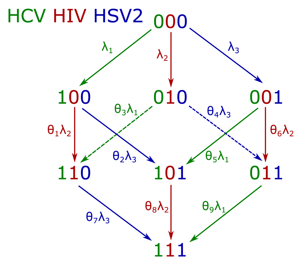
The schematic shows individuals moving between uninfected (0) and infected (1) for each of the infections: HCV; HIV; and HSV2, in that order. The rates of infection are represented as a varying force of infection, λ's for each disease. Where individuals are already infected with at least one of the viruses, these forces of infection are modified by a factor, θ, which could increase or decrease risk.
In addition to the events shown as arrows in Figure 2, we also include a variable death rate due to disease status. Since the natural death rate affects all disease states equally, without changing the proportions of the cohort in each state, we only need to consider the increase (or decrease) in death rate due to a particular disease status. For example, if infection with HIV increases the rate of death, then we would expect the proportions of the cohort in states 010, 110, 011 and 111 to decrease over time relative to the other states due to this.
We take pijk to be the proportion of the total population that have status i for HCV, j for HIV, and k for HSV2. So, for example, p011 is the proportion of the population that are negative for HCV and positive for both HIV and HSV2. Then our model is given by the following ordinary differential equations (ODEs):
where and . Here δHCV and δHIV represent the additional risk of death due to infection with HCV and HIV, respectively.
Note that since we are considering proportions of the total population, the primary way that the additional risk of death is seen in the equations is through the reduction of total population size. This corresponds to an increase in each of the other proportions due to the reduced denominator.
The infection rates (incidences) were allowed to vary smoothly with time and age cohort. This flexible approach allows trends in incidence to be inferred from the data. The parameters are estimated in a Bayesian framework using an adaptive Markov chain Monte Carlo algorithm30 and implemented in R31. The prior for the incidence parameters is a first order Gaussian random walk32, which implies that the difference between incidences at consecutive timepoints/cohorts is Normally distributed with mean zero. This is analogous to a Gaussian process33 evaluated at discrete locations. The variances of the normal distributions describe the smoothness of the incidence surface, and are also estimated from the data. There are six smoothness parameters for each gender and race cohort, one for time and one for age for each of the three viruses. The nine relative risk parameters (the θ’s, see Figure 2) and the initial state of the model in 2003 were also estimated from the data.
We model the proportion of individuals with each infection status separately for each age cohort: birth year before 1943, and then each subsequent birth year up to 1995. We take a Bayesian non-parameteric approach and estimate the three infection rates (incidences) for each year of the study (2003 to 2013) and for each age cohort. We therefore produce three incidence surfaces across time and age cohort. Because there is only a small amount of data for each cohort, we assume that the incidence surfaces are smooth, and so they can “borrow strength” from neighbouring points. Although estimating these incidence surfaces is the main challenge of the inference, in addition we must also estimate the 9 relative risk parameters (θ1, . . . θ9), the initial conditions for each age cohort and the hyperparameters that describe the smoothness of the incidence surfaces.
More precisely, let λi,j,k represent the rate of infection for disease i in year j for age cohort k, for i ∈ {1, 2, 3}, k ∈ K and j ∈ {2003,..., 2015} ∩ Ak, where K is the index set of age-cohorts and Ak is the set of study years after which cohort k reaches 18 years-old. The infection rates can be interpreted as the proportion of a completely susceptible population that would be infected in a year, and therefore we refer to them as incidences. Since we have data at the yearly resolution, we assume that the incidence is constant within each year.
Let represent the vector of initial conditions for age-cohort k, which must sum to 1. These vectors represent either the disease status at the start of the study in 2003; or, for the younger cohorts, the disease status when the cohort turns 18.
Priors. We assume a first order Gaussian random walk prior for the incidences across both time and age-cohort. For all i ∈ {1, 2, 3},
This definition includes 6 hyperparameters (κ’s) that control the smoothness of the surfaces. We assumed that independent Gamma distributed priors with shape parameter 1 and rate parameter 0.01. Since this Gaussian random walk prior only specifies the differences between the lambdas, we also assumed that the mean level of each incidence surface follows an exponential distribution with mean 1%, to provide a mild shrinkage effect on the mean incidences.
The priors for the initial conditions were assumed to be Dirichlet distributions (which ensures that they sum to 1) with parameters equal to α = 0.8/8, following the uninformative prior suggested by Berger et al.34. The priors for the relative risk parameters θ1, . . . θ9 were assumed to be independent exponential distributions with mean 1.
Likelihood. We assumed a multinomial likelihood function. Let be the number of individuals that tests indicate are in disease state m ∈ {(000), (001), . . . , (111)} in year j from age-cohort k. Let dj,k represent the data vector for cohort k in year j and θ represent the complete vector of parameters. To evaluate the likelihood for cohort k in year j we start with the initial conditions pk and solve the differential Equation (1)–Equation (8) forward in time until year j, call this pk(j). This was done using the rk4 Runge-Kutta differential equation solver from the R package deSolve35. The log likelihood of observing data dj,k given pk(j) is simply .
The complete log likelihood is then just the sum over all these component parts.
Markov chain Monte Carlo algorithm. To draw samples from the posterior distribution of the model we used Markov chain Monte Carlo. To update the λi,j,k we used two kinds of single-site proposal. For j and k not on the boundaries we used conditional prior proposals36 for 50% of the updates. For all remaining updates we used a Metropolis-Hastings Gaussian random walk, with proposal variance automatically tuned to 44% by rescaling by a factor xn at iteration n when the iteration is accepted, and by when iteration n is rejected. To achieve diminishing adaptation, we used the sequence xn = 1 + 20/(20 + 0.2n). The precision parameters controlling the smoothness were updated using a Gibbs step.
If we consider only the data for the initial time point, the vector of initial conditions for cohort k, pk, has full conditional distribution pk|d1,k ~ Dir(α1 + d1,k). For the final cohort there is no subsequent data and so the full conditional can be used as a Gibbs step. For earlier cohorts we cannot evaluate the posterior without first solving the system of differential equations. To find an efficient proposal we developed our own adaptive algorithm for Dirichlet distributions (similar to the algorithm in 37) that balances the above conditional distribution against the current location of the chain. Our proposal for pk was ~ Dir(α1 + d1,k + βkpk), which was then accepted or rejected based on the usual Metropolis-Hastings ratio. To find an appropriate value for βk for each cohort k, we applied the following adaptation algorithm during the burn-in phase of the MCMC. If a proposal was accepted then βk ↦ max{0, βk − 3}, and if a proposal was rejected then βk ↦ βk + 1. This leads to an acceptance rate for pk of roughly 25%, unless there is little data after the initial condition, in which case βk ≈ 0 and the acceptance rate is much higher.
The relative risk parameters θ1,..., θ9 were updated with single site Gaussian random walk proposals. To improve the mixing between these highly correlated parameters, we also added a joint update of the θ’s and the means of the 3 incidence surfaces using a Metropolis-Hastings Gaussian random walk in 12 dimensions, with the proposal covariance estimated adaptively using the approach of 30, implemented using the accelerated shaping algorithm38.
Figure 3 shows the posterior median incidence rates in uninfected individuals for the three diseases as a function of time and age-cohort, with lower and upper confidence intervals shown in Figures S2, S3 and S4 (Extended data39). For most groups and most infections we see a much stronger age-cohort effect than a time effect. That is, incidence in a cohort of individuals born in the same year remains approximately constant over time, while an overall decrease in incidence results from lower incidence in younger age groups. This effect is particularly prominent in HCV in black females, black males and white males and in HIV infection in black females (Figure 3). Incidence of all three infections is generally higher in the black population (the first and third rows in Figure 3) than the white population (rows two and four). In most graphs we see a small increase in incidence in the youngest age group in the most recent year. However, this is likely to be a statistical artefact resulting from increasing uncertainty due to fewer age groups (and thus less data) in more recent years. This increase in uncertainty when incidence rates are low can lead to an increase in the median, and so the uncertainty in the estimates is important in these regions (see Figures S1, S2 and S3 of the Extended data for confidence intervals39).
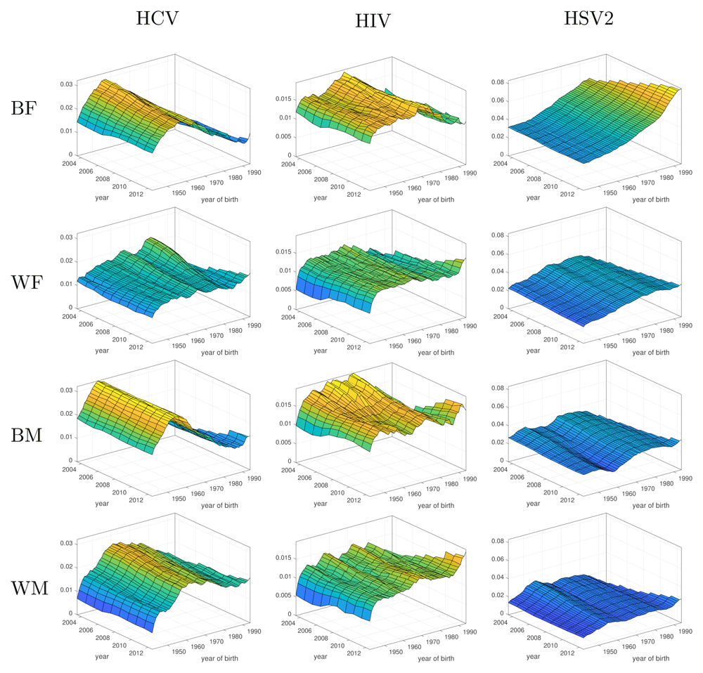
Inferred incidence rates of Hepatitis C Virus (HCV), Human Immunodeficiency Virus (HIV) and Herpes Simplex Virus (HSV2) infection amongst black females (BF), white females (WF), black males (BM) and white males (WM) as a function of time and year of birth.
The first column of Figure 3 shows HCV incidence. Black females, black males and white males all display a strong cohort effect, with individuals born around 1960 experiencing consistently high incidence, while younger cohorts show progressively lower incidence. The posterior median annual incidence peaks at 3.22% (90% CI: 1.66 – 4.76%) in 2003 for black males born in 1953. The peak incidence for black females was 2.95% (1.45 – 4.42%) for those born in 1957 and 2.63% (1.35 – 4.06%) for white males born in 1961, both also in the earliest year in the study. In contrast white females have consistently low incidence, decreasing in all cohorts to between 1.09 and 1.87% for the most recent year.
The second column of Figure 3 shows HIV incidence. HIV incidence is more constant than HCV, and is not as smooth. Incidence in black females and white females is quite constant over time with posterior median incidences in the ranges 1.04–1.91% and 0.52–1.59%, respectively. However, the younger cohorts of black females appear to display somewhat reduced incidence. There is also some indication of reduced incidence in black males in both younger cohorts and more recent years. For black males born in 1962 the posterior median incidence drops from a peak of 1.94% at the start of the study to 1.40% in 2012; however, these declines are small compared to the level of noise (see Figure S2 of the Extended data for HIV confidence intervals39).
The third column of Figure 3 shows posterior median HSV2 incidence. Black females show increasing incidence of HSV2 for later birth cohorts, peaking at 8.34% (90% CI: 5.09–11.5%) in the latest cohort, although there is some suggestion of decreasing risk over time for each cohort. This indicates a higher risk for younger individuals, but decreasing slightly as they age. In contrast, white females’, black males’ and white males’ incidence of HSV2 does not change as much as for black females. White females also show increasing risk for later born cohorts, with a maximum of 3.82% (2.41–5.16%) for individuals born in 1978 and then a decrease for the most recent cohorts. For each cohort, incidence decreases somewhat over time. A similar effect is seen in black males, with the highest-risk cohort born in 1973 with an incidence of 3.61% (1.99–5.26%) and general decreasing incidence over time for each cohort. Black males also display a low-risk cohort born around 1960, with incidence dropping to 1.81% (0.51–3.34%) for those born in 1958. Incidence in white males again shows decreasing risk over time for each cohort and relatively flat incidence between the cohorts.
Table 3 shows the posterior values of the θ parameters (see Figure 2). These give the relative risk of acquiring an infection for individuals that already have another infection. For example, θ1 gives the relative risk of acquiring HIV for individuals that already have HCV. If θ1 > 1 (or θ1 < 1) then this would indicate that individuals with HCV are more likely (less likely, respectively) to acquire HIV than uninfected individuals.
Individuals that already have HSV2 are at lower risk of acquiring HIV or HCV (θ5 and θ6 < 1). This has the possible explanation that individuals that are infected with HSV2 before any other disease are not therefore at high risk of acquiring HIV or HCV. Conversely, individuals that acquire HIV or HCV first are at greater risk of becoming infected with HSV2 (θ2 and θ4 > 1). For those individuals eventually coinfected with HIV and HSV2, if they are infected with HIV first, they rapidly become infected with HSV2. The parameter θ7 represents a similar mechanism, however due to infrequent occurrence of coinfection with both HIV and HCV (due to high death rates), there is insufficient evidence to determine whether θ7 is greater than or less than 1.
The other θ parameters are mostly inconclusive, but there is a suggestion of reduced infection with HIV when already infected with HCV (θ1 < 1), reduced infection with HIV when already infected with both HCV and HSV2 (θ8 < 1) and increased infection with HCV when already infected with both HIV and HSV2 (θ9 > 1).
We extended the random walk prior on the incidences to predict the incidences from 2014 to 2016, with associated uncertainty. The model equations were then solved from 2013 onwards to produce the posterior predictive distribution of prevalences in 2016 with the data from 2016 held-out for validation purposes.
Projections for 2016 were generally quite good for HCV and HIV (bottom rows of Figure 4, Figure 5, Figure 6 and Figure 7, whilst in general overestimating for HSV2. For white males and females the HIV prevalence was very low and the prevalence was overestimated in 2016.
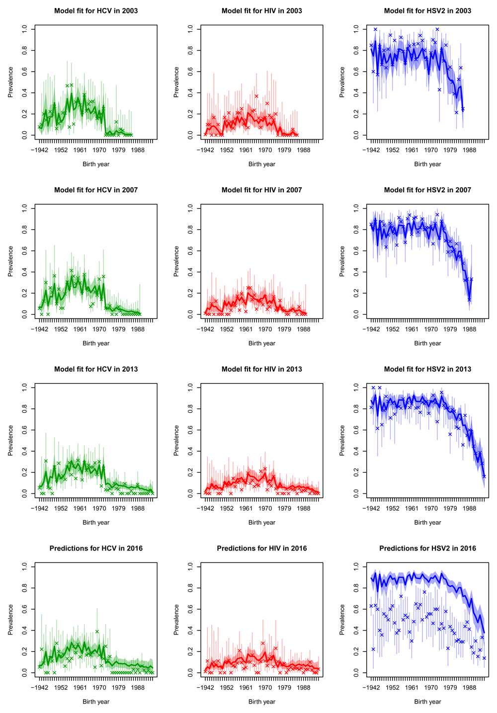
Posterior median prevalence for black females (solid line) and 90% credible intervals (shaded) line for three diseases (columns) in the four sero-surveys (rows), each separated by age cohort. The model has been fitted to the observed data (crosses) in the first three rows of plots but data in the bottom row was held-out for validation purposes. Vertical lines represent 90% binomial CI for the observed data.
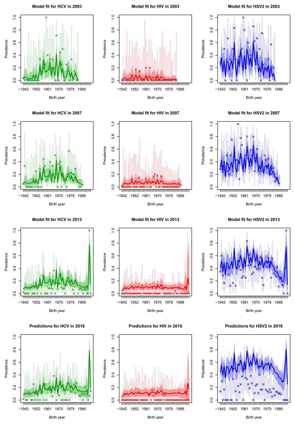
Posterior median prevalence for white females (solid line) and 90% credible intervals (shaded) line for three diseases (columns) in the four sero-surveys (rows), each separated by age cohort. The model has been fitted to the observed data (crosses) in the first three rows of plots but data in the bottom row was held-out for validation purposes. Vertical lines represent 90% binomial CI for the observed data.
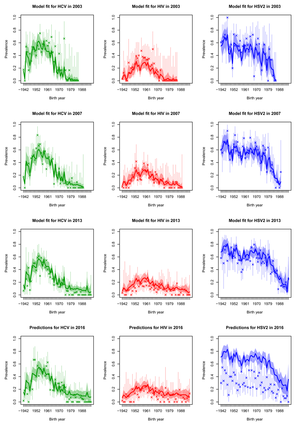
Posterior median prevalence for black males (solid line) and 90% credible intervals (shaded) line for three diseases (columns) in the four sero-surveys (rows), each separated by age cohort. The model has been fitted to the observed data (crosses) in the first three rows of plots but data in the bottom row was held-out for validation purposes. Vertical lines represent 90% binomial CI for the observed data.
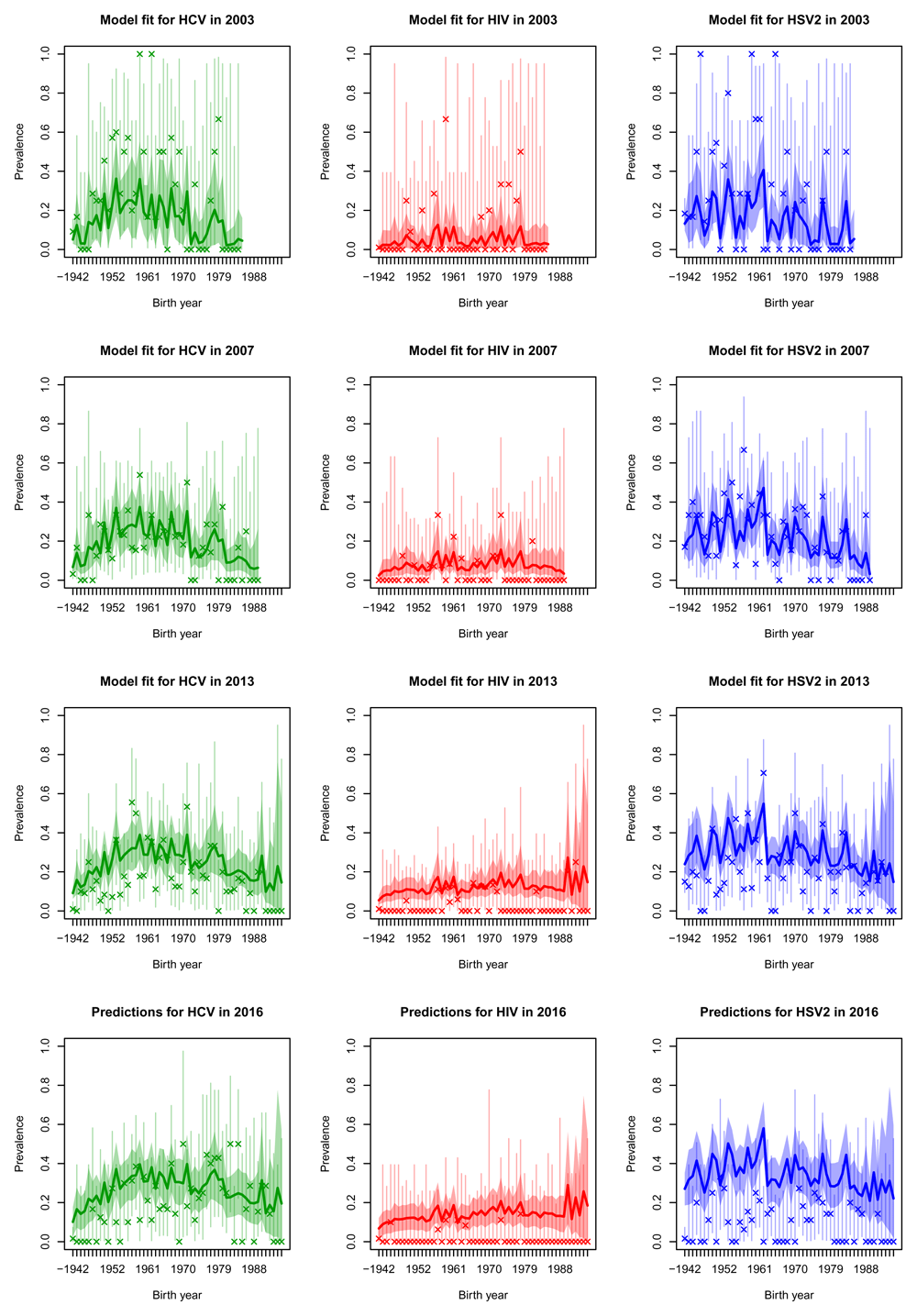
Posterior median prevalence for white males (solid line) and 90% credible intervals (shaded) line for three diseases (columns) in the four sero-surveys (rows), each separated by age cohort. The model has been fitted to the observed data (crosses) in the first three rows of plots but data in the bottom row was held-out for validation purposes. Vertical lines represent 90% binomial CI for the observed data.
Incidence of infections, particularly stratified by key demographic variables, are an essential tool in developing effective control policies, planning for future treatment demand and targeting services. However, direct estimation of incidence of infections like HIV, HCV and HSV2 are almost impossible with current surveillance systems, and even tracking new diagnoses can hide underlying patterns due to changes in health-seeking behaviour in such long-lived infections. Therefore, methods for estimating incidence indirectly are an essential part of the toolbox of understanding these infections. Here we have developed a method of estimating incidence from a relatively cheap and infrequent survey design in a dynamic population of at-risk individuals.
By fitting our model within a Bayesian framework we have been able to fully characterise the uncertainty involved in this estimation procedure. We let the incidences vary smoothly in time and by age cohort, to enable us to borrow strength from similar data to reduce uncertainty, while at the same time providing distinct estimates for each age-cohort through time. This is illustrated in Figure 4, where the uncertainty surrounding the prevalences is much smaller than the binomial CI surrounding the data, in which each observation is treated independently. We applied smoothing to the incidences but not to the initial prevalence distributions, which sometimes leads to noisy prevalence estimates (see Figure 5 in particular). If smoothed estimates of prevalence are required a smoothing penalty prior could be used in place of the independent Dirichlet priors on the initial conditions.
Our study is of a population with a greater burden of HCV, HIV and HSV2 infection than the general population of the United States16,40–42. Data on the prevalence and incidence of these infections in the general Baltimore City population are limited. The observed declines in HCV incidence in young black males and females are consistent with reported declines in HCV incidence in a predominantly-black cohort of community-based people who inject drugs in Baltimore43. In addition, and consistent with our model-based estimates, the observed incidence of HCV between 2003 and 2016 was significantly higher in white ED patients as compared to black ED patients44. The observed declines in HCV incidence in young black populations compared to white populations were also seen recently in New York City (NYC)45. The extremely high incidence in HSV2 and/or HCV after HIV infection is also supported by another finding that shows a very small percentage of women in NYC are infected with HIV only46.
A feature of our estimates is that incidence of disease at a particular age and time is heavily influenced by year of birth. One could speculate that this could indicate a strong impact on behaviour from early influences47,48, or through the behaviour of individuals of a similar age who socialise together49. This emphasises the potential importance of age-cohort counselling and early intervention with peers.
In addition to estimating incidence between surveys, we were able to forward-project from the 2013 survey to the 2016 data, to which the model was not fitted, with moderate success. Our predictions for HCV and HIV were generally good, but the predictions for HSV2 appeared to systematically overestimate the prevalence by a substantial margin. This large change in prevalence across all ages and ethnicities (Figure 1) is thought to be due to changes in the surveyed population, for example due to the implementation of the Affordable Care Act (ObamaCare) in 2014, but this did not seem to have a strong effect on the prevalence of the other diseases. Whilst the results show that incidence rate trends were not constant over this three-year time-period, nevertheless the estimates would have provided useful predictions for public health policy. These forward projections would not have been possible from the prevalence data alone, but required the fitting of a model to the data to estimate incidence rates by age and sex.
The dynamics, incidence and prevalence of coinfection across diseases with similar or related pathways of transmission are an ongoing challenge for surveillance and control. In our analysis of these coinfection data we were able to estimate rates of individual infections after the initial infection; however, there are very few studies with the breadth of coinfection data which is present in this dataset, allowing such an analysis.
The main strength of our approach was that we were able to infer cohort-specific incidence rates that varied through time, and therefore were able to identify trends in incidence at the age, gender and race cohort level. Our results showed that there could be large differences in incidences between age cohorts, which may not have been noticeable from a more naive analysis of the data.
A key weakness of our method was that for our incidence rates to be well-calibrated, we require an accurate estimate of the death rates in HIV and HCV infected populations, over and above the death rate in uninfected populations. This is because the death rates and infection rates are not both identifiable from the proportion of individuals in each infection state. The death rates proved challenging to obtain from the literature, particularly as HIV death rates may have improved substantially in recent years. Nonetheless, if these death rates are stable but incorrectly estimated, any qualitative trends in incidence informed from the data will remain correct.
We have developed a method for estimating age-specific incidence from anonymized cross-sectional prevalence surveys. This approach adds value to the data by providing age and time-specific incidence estimates which could not be obtained any other way and allows forecasting of future incidence. Our findings highlight a cohort-based trend that emphasizes the importance of age-cohort counselling and early intervention at a young age.
Zenodo: drsimonspencer/HIV-HCV-HSV2-coinfection: Source code and extended data. https: //doi.org/10.5281/zenodo.507827139.
This project contains the following underlying data:
Zenodo: drsimonspencer/HIV-HCV-HSV2-coinfection: Source code and extended data. https: //doi.org/10.5281/zenodo.507827139.
This project contains the following extended data:
Data are available under the terms of the Creative Commons Zero ”No rights reserved” data waiver (CC0 1.0 Public domain dedication).
Source code available from: https://github.com/drsimonspencer/HIV-HCV-HSV2-coinfection
Archived source code at time of publication: https://doi.org/10.5281/zenodo.507827139
License: GNU General Public Licence version 3
| Views | Downloads | |
|---|---|---|
| Gates Open Research | - | - |
|
PubMed Central
Data from PMC are received and updated monthly.
|
- | - |
Is the work clearly and accurately presented and does it cite the current literature?
Partly
Is the study design appropriate and is the work technically sound?
Yes
Are sufficient details of methods and analysis provided to allow replication by others?
Yes
If applicable, is the statistical analysis and its interpretation appropriate?
Yes
Are all the source data underlying the results available to ensure full reproducibility?
Yes
Are the conclusions drawn adequately supported by the results?
Yes
References
1. Looker KJ, Elmes JAR, Gottlieb SL, Schiffer JT, et al.: Effect of HSV-2 infection on subsequent HIV acquisition: an updated systematic review and meta-analysis.Lancet Infect Dis. 2017; 17 (12): 1303-1316 PubMed Abstract | Publisher Full TextCompeting Interests: No competing interests were disclosed.
Reviewer Expertise: Biostatistics and infectious disease epidemiology
Is the work clearly and accurately presented and does it cite the current literature?
Yes
Is the study design appropriate and is the work technically sound?
Yes
Are sufficient details of methods and analysis provided to allow replication by others?
Yes
If applicable, is the statistical analysis and its interpretation appropriate?
Yes
Are all the source data underlying the results available to ensure full reproducibility?
Yes
Are the conclusions drawn adequately supported by the results?
Yes
Competing Interests: No competing interests were disclosed.
Reviewer Expertise: Clinical Infectiouis Diseases, mostly HIV and HCV
Alongside their report, reviewers assign a status to the article:
| Invited Reviewers | ||
|---|---|---|
| 1 | 2 | |
|
Version 1 02 Aug 21 |
read | read |
Provide sufficient details of any financial or non-financial competing interests to enable users to assess whether your comments might lead a reasonable person to question your impartiality. Consider the following examples, but note that this is not an exhaustive list:
Sign up for content alerts and receive a weekly or monthly email with all newly published articles
Register with Gates Open Research
Already registered? Sign in
If you are a previous or current Gates grant holder, sign up for information about developments, publishing and publications from Gates Open Research.
We'll keep you updated on any major new updates to Gates Open Research
The email address should be the one you originally registered with F1000.
You registered with F1000 via Google, so we cannot reset your password.
To sign in, please click here.
If you still need help with your Google account password, please click here.
You registered with F1000 via Facebook, so we cannot reset your password.
To sign in, please click here.
If you still need help with your Facebook account password, please click here.
If your email address is registered with us, we will email you instructions to reset your password.
If you think you should have received this email but it has not arrived, please check your spam filters and/or contact for further assistance.
Comments on this article Comments (0)